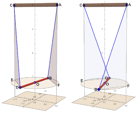
A bifilar pendulum, also known as a "doubly suspended pendulum" is a mechanical system consisting of a uniform rod (labeled as DB in the drawing below) suspended from two parallel wires or filars (AB and CD). These filars allow the rod to rotate freely about the z-axis, with the bob' s movement restricted to rotation and translation along this axis. In other words, the center of mass of the bob stays on the z-axis, and the bob remains level as it rotates. The bob' s rotation is not externally driven, and it is limited to between +/-180 degrees. The bob is considered to be released from an initial position theta0, with an initial angular speed of theta'(0) = 0. Bifilar pendulums can be used to measure the moment of inertia of complex objects such as small boats or model airplanes. By measuring the period of oscillation of the pendulum, one can calculate the moment of inertia of the object suspended from the filars.
Geometry
These are parameters :
theta(t) : angular position (yaw) of the bob bar around the z-axis
h(t): vertical position of the bob bar
d: half the spacing of the parallel suspension lines and half the length of the bob bar
f: length of the 2 suspension lines (f > 2d)
L: height of top bar above the x - y plane h: vertical displacement of the bob bar along the z-axis
M: moment of inertia; V: potential energy; T: kinetic energy
In one of the two right triangles AFB or CED:
BF1 = Sqrt[f^2 - h^2];
In the isosceles triangle OBF:
BF2 = 2 d Sin[theta/2];
Quiet@Last@SolveValues[BF1 == BF2, h] // Simplify
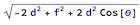
The previous formula is the relation between the rotational (theta) and translational (h) displacement of the bob. It is used to find the equation of motion.
Equation of Motion: using Lagrangian mechanics.
h[t_] := Sqrt[-2 d^2 + f^2 + 2 d^2 Cos[theta[t]]];
(*potential energy*)V = m g (L - h[t]);
(*moment of inertia of a thin rod of length 2d and mass \
m,perpendicular to the axis of rotation,rotating about its center.*)
M = 1/3 d^2 m ;
(*kinetic energy due to rotation around z-axis*)
Trot = 1/2 M theta'[t]^2;
(*kinetic energy due to translation along z-axis*)
Ttrn = 1/2 m  h'[t]^2;
(*total kinetic energy*)T = Trot + Ttrn;
(*Lagrangian*)Lgr = T - V // Simplify;
(*equation of motion*)deqn =
 Apply[D[ D[Lgr, #1], t] - D[Lgr, #2] == 0 & , {{theta'[t],
     theta[t]}}, 1] // FullSimplify
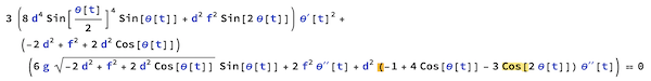
Based on the above, the angular displacement function can be defined for the bifilar pendulum.
thetaSol[theta0_, f_, d_] :=
 With[{g = 9.81},
  NDSolveValue[{3 (8 d^4 Sin[theta[t]/2]^4 Sin[theta[t]] +
         d^2 f^2 Sin[2 theta[t]]) Derivative[1][theta][
        t]^2 + (-2 d^2 + f^2 +
         2 d^2 Cos[theta[t]]) (6 g Sqrt[-2 d^2 + f^2 +
           2 d^2 Cos[theta[t]]] Sin[theta[t]] +
         2 f^2 (theta^\[Prime]\[Prime])[t] +
         d^2 (-1 + 4 Cos[theta[t]] - 3 Cos[2 theta[t]]) (
           theta^\[Prime]\[Prime])[t]) == 0, theta[0] == theta0,
    theta'[0] == 0}, theta, {t, 0., 32}]]
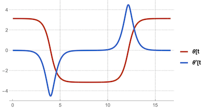
This plot shows the evolution of the angular displacement and -speed for one period and with an initial displacement theta0 close to the maximum Pi:
With[{f = 6., theta0 = Pi - .001},
 Plot[Evaluate[{thetaSol[theta0, f, 1.][t],
    D[thetaSol[theta0, f, 1.][t], t](*,D[thetaSol[theta0,f,1][t],{t,
    2}]*)}], {t, 0, 16.6}, Frame -> True, FrameLabel -> "t",
  PlotLegends -> {"\[Theta][t", "\[Theta]'[t", "\[Theta]''[t"},
  GridLines -> Automatic, PlotTheme -> "Web"]]
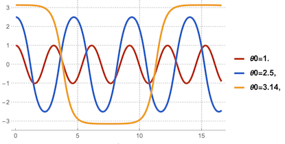
This is the dependence of theta on the initial displacement theta0:
With[{f = 6.},
 Plot[Evaluate[thetaSol[#, f, 1.][t] & /@ {1., 2.5, 3.14}], {t, 0,
   16.6}, Frame -> True, FrameLabel -> "t",
  PlotLegends -> {"\[Theta]0=1.", "\[Theta]0=2.5,",
    "\[Theta]0=3.14,"}, GridLines -> Automatic, PlotTheme -> "Web"]]
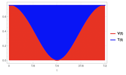
Energy conservation
To verify the equation of motion for the bifilar pendulum, it is important to check whether the energy in the system is conserved. This can be done by plotting the exchange of potential and kinetic energy during e.g. one half period of the pendulum's motion.
Block[{V, M, T, g = 9.81, L = 6, f = 6, d = 1, theta0 = 1., m = 1,
  tMax = 24, h, pf},
 pf = periodFull[theta0, f, d];
 h[t_] := Sqrt[-2 d^2 + f^2 + 2 d^2 Cos[thetaSol[theta0, f, d][t]]];
 V[t_] := g m (L - h[t]); M = m d^2/3;
 T[t_] :=(*rotational*)
  1/2 M   D[thetaSol[theta0, f, d][t], t]^2 +(*translational*)
   1/2 m  h'[t]^2;
 Plot[Evaluate@{V[t], V[t] + T[t]}, {t, 0.,
   periodFull[theta0, f, d]/2}, Frame -> True, FrameLabel -> "t",
  FrameTicks -> {{Automatic,
     None}, {Transpose[{pf/2 Range[0, 1, .25], {"0", "T/8", "T/4",
        "3T/8", "T/2"}}], None}}, PlotRange -> All,
  PlotLegends -> {"V(t)", "T(t)"}, Filling -> {2 -> Axis, 1 -> {2}},
  FillingStyle -> {Blue, Red}]]
Video GIF
The equation of motion for the bifilar pendulum can be visualized through GIF animations. This video shows the pendulum's motion under different initial displacement angles. The left video shows a pendulum with an initial displacement angle of 110 degrees, while the right video depicts the pendulum at its maximum initial displacement angle of 180 degrees.
frames =
  ParallelTable[
   Block[{ptA, ptB, ptC, ptD, h, L = 5, f = 4, theta0 = 2.(*3.*)},
    ptA = {1, 0, L};
    h = Sqrt[-2 + f^2 + 2 Cos[thetaSol[theta0, f][time]]];
    ptC = {-1, 0, L};
    ptB = RotationTransform[thetaSol[theta0, f][time], {0, 0, 1}][{1,
       0, L - h}];
    ptD = RotationTransform[thetaSol[theta0, f][time], {0, 0, 1}][{-1,
        0, L - h}];
    Graphics3D[{{Brown,
       Cylinder[{{0, 0, 0}, {0, 0, 0.1}}, 1.65 ]}, {AbsoluteThickness[
        4], Line[{{1.5 , 0, L}, {1.5 , 0, 0}}],
       Line[{{-1.5 , 0, 0}, {-1.5 , 0, L}}]}, {Brown,
       Cylinder[{{1.6 , 0, L}, {-1.6 , 0, L}}, .075]}, {Blue,
       AbsoluteThickness[1.5], Line[{ptA, ptB}],
       Line[{ptC, ptD}]}, {Red,
       Cylinder[{ptB, ptD}, .05]}, {AbsolutePointSize[8],
       Point[{ptB, ptD}]}}]], {time, 0, 3.182, 3.182/50}];
Export[NotebookDirectory[] <> "video.GIF", frames]
Different suspension line lengths can be compared, ranging from 5d to the left to the minimum of 2d to the right.
Period
The function WhenEvent can be used to detect the times when the pendulum reaches zero speed at its turning points. The period can be computed by differentiating this times.
periodReal[theta0_, f_, d_ : 1] :=
 2 First[Differences[
    Last[Last[
      With[{g = 9.81},
       Reap[NDSolveValue[{3 (8 d^4 Sin[theta[t]/2]^4 Sin[theta[t]] +
               d^2 f^2 Sin[2 theta[t]]) Derivative[1][theta][
              t]^2 + (-2 d^2 + f^2 +
               2 d^2 Cos[theta[t]]) (6 g Sqrt[-2 d^2 + f^2 +
                 2 d^2 Cos[theta[t]]] Sin[theta[t]] +
               2 f^2 (theta^\[Prime]\[Prime])[t] +
               d^2 (-1 + 4 Cos[theta[t]] - 3 Cos[2 theta[t]]) (
                 theta^\[Prime]\[Prime])[t]) == 0, theta[0] == theta0,
           Derivative[1][theta][0] == 0,
          WhenEvent[Derivative[1][theta][t] == 0., Sow[t]]},
         theta, {t, 0., 32}]]]]]]]
The following plot shows the dependence of the period on the starting position theta0 for different lengths f of the suspension lines. The real period (colored lines) differs only slightly from the simplified one (dashed lines based on formula below) for an angular displacement up to 30 degrees.
tbl[L_] :=
 Table[{t0, periodReal[t0, L]}, {t0, .1, 3.14, .05}]; lst = {2, 4, 10,
   20, 50};
Module[{g = 9.81},
 ListLinePlot[Evaluate[tbl /@ lst], PlotStyle -> AbsoluteThickness[3],
   Frame -> True, GridLines -> {Range[0, 180 °, 15 °], Automatic},
  FrameTicks -> {{Automatic, None}, {Range[0, 180 °, 15 °], None}},
  FrameLabel -> {"\[Theta]0", "T (sec)"},
  PlotLegends ->
   Reverse[{"\[ScriptL]=2", "f=4", "f=10", "f=20", "f=50"}],
  Epilog -> {Dashed,
    Line[({{0, (2 Sqrt[(#1 m)/3] \[Pi])/(Sqrt[g] Sqrt[m])}, {1.5, (
          2 Sqrt[(#1 m)/3] \[Pi])/(Sqrt[g] Sqrt[m])}} &) /@ lst]}]]

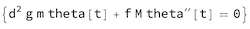
Simplified Equation of Motion for small angular displacement
As shown on the previous plot, for most practical applications, one can simplify the equation of motion for small displacement of the bob:
simpleRule = {Cos[_] -> 1, Sin[t_] -> t}; Clear[M];
T = 1/2 M theta'[t]^2; Lgr = T - V;
deqnSimple =
 Apply[D[ D[Lgr, #1], t] - D[Lgr, #2] == 0 & , {{theta'[t],
      theta[t]}}, 1] /. simpleRule // Simplify[#, f > 2 d > 0] &
A simplified equation can be derived for the period and the moment of inertia.
First@DSolve[deqnSimple, theta, t]

The period from the function above is the pendulum period for the case of small displacements:
Quiet@First@
   SolveValues[(d Sqrt[g] Sqrt[m] )/(Sqrt[f] Sqrt[M]) == 2 Pi/Ts,
    Ts] // Simplify[#, {f > 2 > 0}] &

This is the moment of inertia for the case of small displacements. It is the formula frequently used in experiments to find the moment of inertia of a complicated object.
Quiet@First@
   SolveValues[(d Sqrt[g] Sqrt[m] )/(Sqrt[f] Sqrt[M]) == 2 Pi/Ts, M] //
  Simplify[#, {f > 2 > 0}] &


