The Emil Post Tag System Explained
Post's tag system, is one deterministic computational model that was developed by Emil Post, the American logician and mathematician. Millions of mathematicians, computer scientists, and theoretical physicists alike view the elegant emergence of deterministic behavior from simple rules, and they all appreciate how great it is. As a source of profound insights into the nature of computation and complexity, the abstract computational devices of Post among which are the Turing Machine and Cellular Automata, are really about the works of string re-writing. So when you're beach-balling and back-filling computational holes, you never know when you might need to push the boundaries of our understanding, whether it's computational rules that seem unrelated, or it's the unanticipated connection that we discover on our map to universality..our understanding of the computational universe serves as an evocative and vivid reminder of the inherent advantage and profound depth of seemingly simple mathematical constructs. What are they? When you drill down to the foundations of computability theory you'll find some Tag machines in them, that continue to emulate the principle of universal computation. The computational universe described by the Ruliad is limitless and manifold. Navigating it can be a daunting task! What with all the things the computational explorer encounters..however, that's what happens when you systematically leverage the powers of computationally irreducible, symbolic landscapes of emergent, complex phenomena. As they unfold.
rules1 = {
   {left___, 0, 0, s___} :> {left, s, 0, 1, 1},
   {left___, 1, 0, s___} :> {left, s, 1, 0},
   {left___, 0, 1, s___} :> {left, s, 0, 1, 1},
   {left___, 1, 1, s___} :> {left, s, 1, 0}};
rules2 = {
   {left___, 0, 0, s___} :> {left, s, 0, 0},
   {left___, 1, 0, s___} :> {left, s, 1, 0},
   {left___, 0, 1, s___} :> {left, s, 0, 1},
   {left___, 1, 1, s___} :> {left, s, 1, 1}};
rules3 = {
   {left___, 0, 0, s___} :> {left, s, 1, 1, 1},
   {left___, 1, 0, s___} :> {left, s, 0, 0},
   {left___, 0, 1, s___} :> {left, s, 1, 1, 0},
   {left___, 1, 1, s___} :> {left, s, 0, 0, 0}};
rules4 = {
   {left___, 0, 0, s___} :> {left, s, 1, 0, 1, 1, 0},
   {left___, 1, 0, s___} :> {left, s, 0, 1, 0, 0, 1},
   {left___, 0, 1, s___} :> {left, s, 1, 1, 0, 1, 1},
   {left___, 1, 1, s___} :> {left, s, 0, 0, 1, 0, 0}};
rules5 = {
   {left___, 0, 0, s___} :> {left, s, 1, 0, 1},
   {left___, 1, 0, s___} :> {left, s, 0, 1},
   {left___, 0, 1, s___} :> {left, s, 1, 1, 0},
   {left___, 1, 1, s___} :> {left, s, 0, 0}};
rules6 = {
   {left___, 0, 0, s___} :> {left, s, 1},
   {left___, 1, 0, s___} :> {left, s, 0, 1, 0},
   {left___, 0, 1, s___} :> {left, s, 1, 0},
   {left___, 1, 1, s___} :> {left, s, 0, 0, 0}};
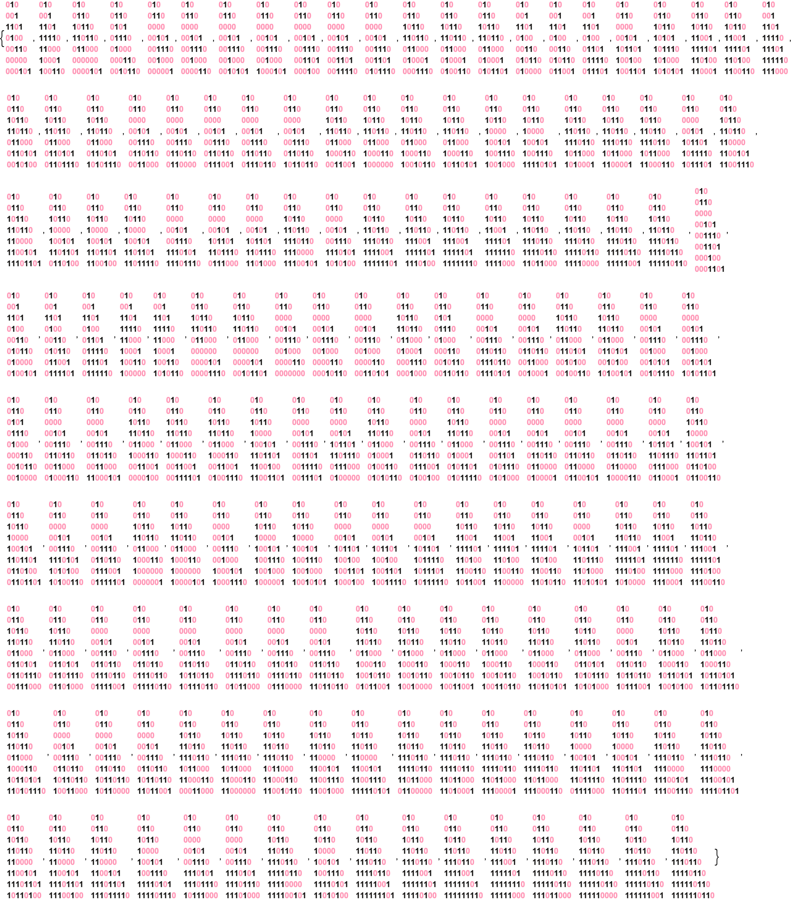
And now that we have these rules defined with all these extra spaces added in there, here's what comes next. There's the pattern symbol _, because when we use the symbol Blank[] or None, or 0, we are following some additional wildcard aspects..part of how this graph got the way it got, is that we follow this enchanting, wildcard pattern for an undirected graph, with a list of vertices, as they are simple entities. It's not just one juncture of time and space, we can also properly configure the kernel for the thrill of parallel computation in any space. You could even construct a gateway to..more complex models and concepts, since NestGraph, the function that is, generates a sequence of graph nests for each timeStep, allowing us not to have to even regenerate the graphs. That's Mathematica. The initial condition that we've got, 101, is constant. It's constant across different timeStep values and as we observe these tag systems in their incredible transformation, the initial condition still holds the value of 101. Furthermore and regardless of the initial condition, the tag system generates promisingly distinct visits; once the algorithm explores the configurations, edges, maximum edges, density ratio, we can also remove vertices of the multi-way graph from the frontier, the queue and add vertices to the back, of the queue. If a vertex has been added only once, it is removed, and if an incoming vertex is adjacent then it can be added. When you change the order of the elements, whether or not you reverse the previous rules or make bigger jumps around the Ruliad by replacements or introduce longer replacements, it might take a while to reverse previous rules and make bigger jumps around by replacements and introduce longer replacements. It might take a while, to find something good: these sensational rules, leave it at that: even with small changes these rule sets will produce different kinds of behavior of the construct of multi-way tag systems. The deterministic coordinatized framework, at the request to explain everything about how the world works, how multi-way tag systems interact in defined mathematical spaces..the spacing on the functions we've got to this day we can see how the deterministic coordinatized framework of multi-way tag systems explains how we can extend Emil Post's original tag systems, and play a central role in defining the breadth of computational universality because, assuming that all possible computation type of rules are laid out and defined, that's not actually, not such a good thing..the intricate interaction of multi-way tag systems, is a delectable. Within this complex web of every potential computational outcome at once.
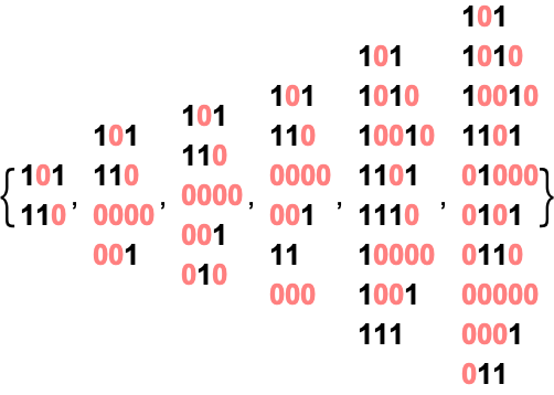
AllGenerationPlotsBinary[g_, minHeight_] := Module[
  {matrices, styledMatrices},
  matrices = Table[PadRight[With[{vertices = VertexList[g],
        randomInit = Tuples[{0, 1}, 3]},
       Table[
        FindShortestPath[g, First[VertexList[g]], vertices[[i]]], {i,
         1, Length[vertices]}]][[j]],
     {Automatic, Automatic}, .25],
    {j, 2, Length[VertexList[g]]}];
  styledMatrices = Map[If[# == 1, Style[#, Bold, Hue[.1, .1, .1]],
      If[# == 0, Style[#, Bold, Hue[.95, .4, 1.4]]]] &, matrices, {3}];
  styledMatrices = Select[styledMatrices, Length[#] >= minHeight &];
  Style[Text[Table[Column[Row /@ styledMatrices[[i]], Left],
     {i, 1, Length[styledMatrices]}]]]]
AllGenerationPlotsBinary[
 NestGraph[ReplaceList[rules1], {{0, 1, 0}}, 7], 7]
AllGenerationPlotsBinary[
 NestGraph[ReplaceList[rules2], {{0, 1, 0}}, 7], 1]
AllGenerationPlotsBinary[
 NestGraph[ReplaceList[rules3], {{0, 1, 0}}, 7], 1]
AllGenerationPlotsBinary[
 NestGraph[ReplaceList[rules4], {{0, 1, 0}}, 3], 1]
AllGenerationPlotsBinary[
 NestGraph[ReplaceList[rules5], {{0, 1, 0}}, 7], 7]
AllGenerationPlotsBinary[
 NestGraph[ReplaceList[rules6], {{0, 1, 0}}, 7], 7]

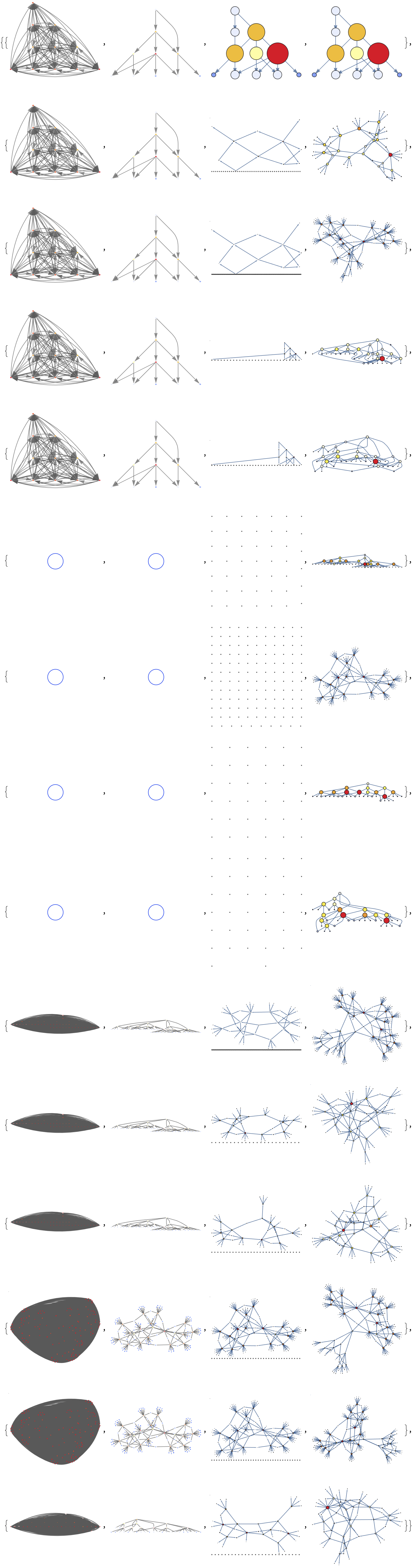
Now that we have our rules, we can get all kinds of cascading patterns. We can generate ListStepPlot. Why is the last time step the only parameter? Because now you know, what the rules are already. The representation of time steps instantaneously represents positions on the Tag system where the values go along with the state of the Tag system, at each time step. The method we visualize the sublime context of the tag systems, which languish behind the real nested structure of the tag systems, it's programmatically possible to explore the various visual representations of the tag system that keeps on computing & generating.
rulesListStepPlot[rules_, lastTimeStep_] :=
 ListStepPlot[
  Legended[
   FlattenAt[
    Table[With[{graph =
        NestGraph[ReplaceList[rules], {{1, 0, 1}}, timeStep,
         VertexShapeFunction -> _ -> (Inset[
              ArrayPlot[{#2}, ImageSize -> 32], #1, #3] &),
         PerformanceGoal -> "Speed"]},
      With[{vertices = VertexList[graph]},
       Style[Text[
           Table[Length /@
             FindShortestPath[graph, First[vertices],
              vertices[[v]]], {v, 1,
             Length[vertices]}]]][[1]][[1]]]], {timeStep, 1,
      lastTimeStep}], {#} & /@ Range[lastTimeStep]], {0, 1, 0}]]
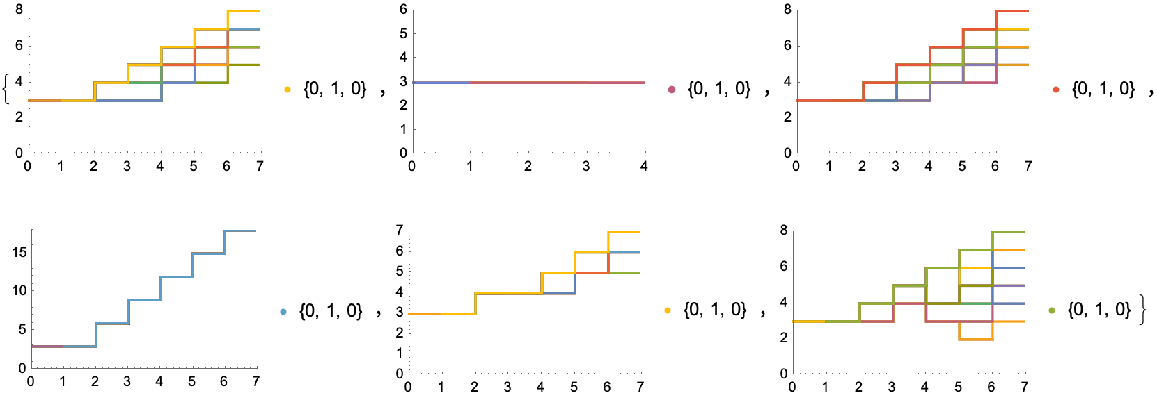
It's possible, for tag systems to emulate the universal Turing Machine and effectively get more universal computation. As seen previously now, how it goes, the ListStepPlot coming up from antiquity, you could try to enhance the computational speed of the plot and do so with ease, via mathematics, or you could accidentally generate a long ListStepPlot that takes ages to load and get this radiant, gorgeous, ListStepPlot by avoiding the redundancy that justifies the fact that it actually exists. Mathematica can perform certain tasks in parallel, making use of all cores of your processor with the processing overhead..the graphs are made of snowflakes, because of this processing.
rules1String = {"00" -> "011", "10" -> "10", "01" -> "011",
"11" -> "10"};
rules2String = {"00" -> "00", "10" -> "10", "01" -> "01",
"11" -> "11"};
rules3String = {"00" -> "111", "10" -> "00", "01" -> "110",
"11" -> "000"};
rules4String = {"00" -> "10110", "10" -> "01001", "01" -> "11011",
"11" -> "00100"};
rules5String = {"00" -> "101", "10" -> "01", "01" -> "110",
"11" -> "00"};
rules6String = {"00" -> "1", "10" -> "010", "01" -> "10",
"11" -> "000"};
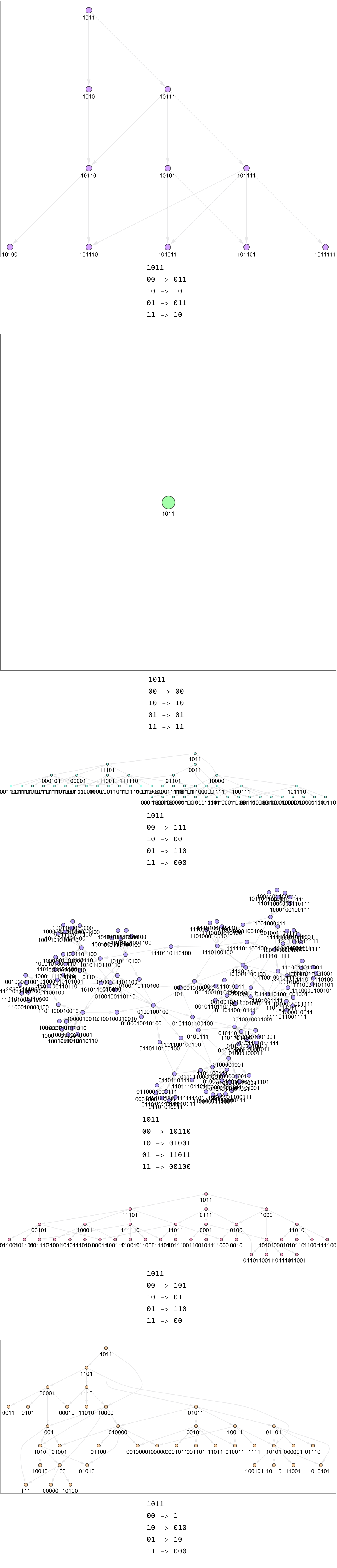
init = {"1011"};
applyRules[rules_, init_] := Module[{rulesTemplate},
rulesTemplate = <|
"init" -> init[[1]],
"v1" -> rules[[1, 2]],
"v2" -> rules[[2, 2]],
"v3" -> rules[[3, 2]],
"v4" -> rules[[4, 2]],
"k1" -> rules[[1, 1]],
"k2" -> rules[[2, 1]],
"k3" -> rules[[3, 1]],
"k4" -> rules[[4, 1]]
|>;
Labeled[Graph[ResourceFunction["MultiwaySystem"][rules, init, 3,
"StatesGraphStructure", VertexLabels -> Placed["Name", Below],
ImageSize -> 600, Frame -> {{True, False}, {True, False}}],
VertexStyle -> {_ -> Hue[RandomReal[], 0.5, 1]},
EdgeStyle -> Directive[Opacity[0.5], Hue[0.8, 0.3, 0.1, 0.1]]],
StringTemplate["`init`\n`k1` -> `v1` \n`k2` -> `v2`
`k3` -> `v3` \n`k4` -> `v4` \n"][rulesTemplate]]]
TableForm[{applyRules[rules1String, init],
applyRules[rules2String, init],
applyRules[rules3String, init],
applyRules[rules4String, init],
applyRules[rules5String, init],
applyRules[rules6String, init]}]
It's intriguing how the tag systems produce sequences for each computational cycle in the beginning and end of the string, this is exhilarating: we can perform a breadth-first search to show how the system continues to evolve according to these rules, rule 1 that is, continuing indefinitely. Of course, there are also systems that repeat a state and, and reach an empty string. Mathematica computes the shortest path repeatedly for each vertex. Unless you've got some complex operations, as long as you're using built-in functions whenever possible, it might be even more expedient and picturesque to compute the list of shortest paths once. Or, if you wish you can do it this way and then compute the shortest path each time, which should free up computational space if all we want is, the shortest path is actually the shortest path..what with what Mathematica provides. It's extraordinary and rare to find a shortest path that isn't predictable..surely if there's a function you know where the size & complexity of the graph are simple, then we could get the metrics like visited nodes, graph density, and these.
metricFN[g_, visitedNodes_, queueSize_] := Module[
  {visitedNodesCount, graphDensityVisited},
  visitedNodesCount =
   Length[Intersection[visitedNodes, VertexList[g]]];
  graphDensityVisited =
   If[visitedNodesCount > 1,
    EdgeCount[g]/(visitedNodesCount*(visitedNodesCount - 1)/2), 0];
  Return[{visitedNodesCount, graphDensityVisited, queueSize}];]
BFS[g_, start_, end_] := Module[
  {parent = <||>, queue = {start}, current, neighbors, path = {},
   queueList = {}, parentList = {}, metricsList = {}},
  While[Length[queue] > 0, current = First[queue];
   queue = Rest[queue];
   neighbors = AdjacencyList[g, current];
   For[i = 1, i <= Length[neighbors], i++,
    If[! KeyExistsQ[parent, neighbors[[i]]],
      parent[neighbors[[i]]] = current;
      AppendTo[queue, neighbors[[i]]];
      If[neighbors[[i]] == end, queue = {}];];];
   AppendTo[queueList, Length[queue]];
   AppendTo[parentList, Length[Keys[parent]]];
   AppendTo[metricsList, metricFN[g, Keys[parent], Length[queue]]];];
  current = end;
  While[current != start, PrependTo[path, current];
   current = parent[current];];
  PrependTo[path, start];
  Return[{path, queueList, parentList, metricsList}];]
visualizeWithBFS[g_, start_, end_] := Module[
  {result = BFS[g, start, end], rangePlot, graphMetricsPlot},
  rangePlot = Rotate[ArrayPlot[
     PadRight[result[[1]], Automatic, 0],
     Frame -> True,
     ColorRules -> {0 -> Hue[.95, .4, 1.4], 1 -> Hue[.1, .1, .1]},
     Mesh -> True], 90 Degree];
  graphMetricsPlot = ListLinePlot[Transpose[result[[4]]],
    PlotRange -> All,
    PlotLegends ->
     Placed[{"Visited Nodes", "Edge Density", "Queue Size"}, Below],
    PlotLabel -> Style["Graph Metrics Over Time", FontSize -> 12],
    PlotTheme -> "Detailed"];
  Return[{rangePlot, graphMetricsPlot}]]
g = ResourceFunction["NestGraphTagged"][ReplaceList[rules1],
   {{0, 0, 1}}, 3,
   VertexShapeFunction -> _ -> (Inset[
        ArrayPlot[{#2}, ImageSize -> 32], #1, #3] &)];
RandomMultiwayTagSystem[g_] :=
 Module[{vertices = VertexList[g], shortestPaths},
  shortestPaths =
   Table[visualizeWithBFS[g, First[vertices], vertices[[i]]], {i, 1,
     Length[vertices]}];
  Grid[Partition[Flatten[shortestPaths], 2, 2, {1, 1}, {}],
   Frame -> All]]
RandomMultiwayTagSystem[g]
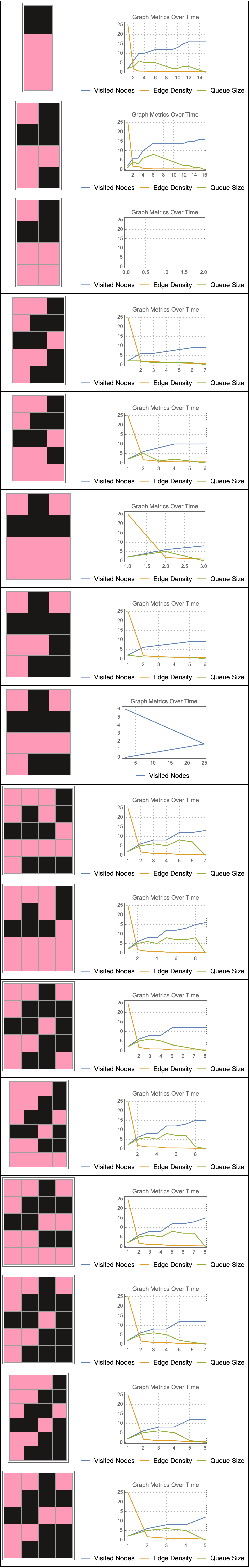
Consider the following. With these fine metrics you can generate multi-way tag system rule 4 in a form that can only be described as a snowflake. I got bewildered finding out how the visited nodes grow as Breadth-First Search "BFS" explores the graph. Inherently with a 3D printer we might keep track of the BFS process more concretely, and see which nodes lead to the discovery of a new node, there are so many of them. It's not hard what the BFS process does; the growth rate of the visited nodes is the gift of insight into the density of the connectivity of the graph, still shy of the complete density of the connected graph, therefore suggests that there's an outstanding queue size over time. The queue sizes are not nothing. In fact they represent the size of the BFS queue at each step; that's why we've got to represent the graph in layers along the scale of a source node and its neighbors, then the neighbors of those neighbors, and so on.
Column[Table[Column[Table[NestGraph[ReplaceList[rule],
     {{0, 1, 0}}, i], {i, 5}]],
  {rule, {rules1, rules2, rules3, rules4, rules5, rules6}}]]

Set a length of the end & beginning of the string; what does this have to do with the complex behavior of tag systems in universal computation? There are a massive amount of neighbors..yarg! I can't believe it. If the queue size says how much node is made at each step, then a rapidly growing queue size might suggest that the graph is on its way to the highest echelons of branching; a small queue size might suggest a more low-degree, linear, mind-boggling structure.
AllGenerationPlotsBinary[g_, len_] :=
 Module[{matrices, styledMatrices, filteredVertices},
  filteredVertices = Select[VertexList[g], Length[#] == len &];
  matrices =
   Table[PadRight[
     With[{vertices = filteredVertices},
       Table[FindShortestPath[g, First[vertices], vertices[[i]]], {i,
         1, Length[vertices]}]][[j]], {Automatic,
      Automatic}, .25], {j, 2, Length[filteredVertices]}];
  styledMatrices = Map[If[# == 1, Style[#, Bold, Black],
      If[# == 0, Style[#, Bold, Pink]]] &, matrices, {3}];
  Style[Text[
    Table[Column[Row /@ styledMatrices[[i]], Left], {i, 1,
      Length[styledMatrices]}]]]]
AllGenerationPlotsBinary[NestGraph[ReplaceList[{
    {left___, 0, 0, s___} :> {left, s, 1},
    {left___, 1, 0, s___} :> {left, s, 0, 1, 0},
    {left___, 0, 1, s___} :> {left, s, 1, 0},
    {left___, 1, 1, s___} :> {left, s, 0, 0, 0}}],
  {{1, 0, 1}}, 10], 3]
This field under the proper care became eventually known as computability theory. It's been delightful, exploring these tag systems within the coordinatized framework. This captivating framework that fills the Rulial Space, how does it function? There is a hole, in the rotated ArrayPlot, where BFS bubbles up. It bubbles up from the start node to the end node, for which each row in this plot corresponds to a step in the path accumulating a list of nodes which were visited at that step. This helps visualize the sequence of nodes visited during the search process. This is so diverse, the BFS stuff that gets buried underground that nobody exactly keeps track of; it's worth something. The BFS algorithm, doesn't change the graph itself! It merely visits the nodes in the right sequence. For instance, when modeling snowflakes I don't really care about the fluffiness of the snowflakes, all I care about, is the growth rate of the arms. Similarly, if there really are some dynamic metrics unknowingly spawned that live as the BFS progresses, then we could compute stuff like the maximum out-degree. We could compute the ratio of leaf nodes. This factor & cluster of graph density thing is really just fabulous, we can do it via the composition of our sub-graphs.
Did we re-factor our code to refer to the specific configurations that exhibit interesting or unique behavior? Yes we did! And it's looking awfully good. It would be even more astonishing to generate halting configurations in a neon color scheme so that we can represent the termination of the tag system, or even the tag systems that enter into infinite loops where they continuously cycle through a set of configurations without reaching, unless they land right-side up on the halting configuration at the end. How can we understand the repetitive behavior of the system?
rulesListString = {{"00" -> "011", "10" -> "10", "01" -> "011",
    "11" -> "10"},
   {"00" -> "00", "10" -> "10", "01" -> "01", "11" -> "11"},
   {"00" -> "111", "10" -> "00", "01" -> "110", "11" -> "000"},
   {"00" -> "10110", "10" -> "01001", "01" -> "11011",
    "11" -> "00100"},
   {"00" -> "101", "10" -> "01", "01" -> "110", "11" -> "00"},
   {"00" -> "1", "10" -> "010", "01" -> "10", "11" -> "000"}};
init = {"1011"};
statesGraphList =
  ResourceFunction["MultiwaySystem"][#, init, 3, "StatesGraph"] & /@
   rulesListString;
statesGraphList =
  Graph[#, VertexLabels -> None,
     VertexShapeFunction -> (Circle[#, 0.02] &)] & /@
   statesGraphList;
evolutionGraphWeightedStructureList =
  ResourceFunction["MultiwaySystem"][#, init, 3,
     "EvolutionGraphWeightedStructure"] & /@ rulesListString;
transformGraphs[graphList_] :=
 Module[{pairs, results = {}, graph1, graph2, complementGraph,
   contractedGraph, differenceGraph, unionGraph, vertices},
  pairs = Subsets[graphList, {2}];
  For[i = 1, i <= Length[pairs], i++, graph1 = pairs[[i, 1]];
   graph2 = pairs[[i, 2]];
   complementGraph = GraphComplement[graph1];
   vertices = VertexList[graph1];
   contractedGraph =
    If[Length[vertices] >= 2,
     VertexContract[graph1, Take[vertices, 2]], graph1];
   differenceGraph = GraphDifference[graph1, graph2];
   unionGraph = GraphUnion[graph1, graph2];
   AppendTo[
    results, {complementGraph, contractedGraph, differenceGraph,
     unionGraph}];];
  results]
statesGraphListTransformed = transformGraphs[statesGraphList];
evolutionGraphWeightedStructureListTransformed =
  transformGraphs[evolutionGraphWeightedStructureList];
drawHeatmapGraph[graph_, densities_] :=
 Graph[graph,
  VertexStyle -> (#[[1]] -> ColorData["TemperatureMap"][#[[2]]] & /@
     Normal[densities]),
  VertexSize -> (#[[1]] -> #[[2]] & /@ Normal[densities])]
normalize[x_List] := If[Max[x] == 0, x, x/Max[x]]
vertexDegreesLists =
  Map[VertexDegree, statesGraphListTransformed, {2}];
vertexDensitiesLists =
  MapThread[
   AssociationThread[
     VertexList[#1] -> normalize[#2]] &, {statesGraphListTransformed,
    vertexDegreesLists}, 2];
MapThread[drawHeatmapGraph, {statesGraphListTransformed,
  vertexDensitiesLists}, 2]
We who are the developers, we just want to reach out and extend our oscillating configurations to understand the periodicity of the system.
What happened to the unreachable configurations? It's been quite a harrowing, boundary and exception accessibility issue that we will just stick here; no need to self-assemble and modify the configurations themselves, that would be a stiff computation.
vertexDegreesLists =
  Map[VertexDegree,
   evolutionGraphWeightedStructureListTransformed, {2}];
vertexDensitiesLists =
  MapThread[
   AssociationThread[
     VertexList[#1] ->
      normalize[#2]] &, \
{evolutionGraphWeightedStructureListTransformed, vertexDegreesLists},
   2];
MapThread[drawHeatmapGraph, \
{evolutionGraphWeightedStructureListTransformed,
  vertexDensitiesLists}, 2]
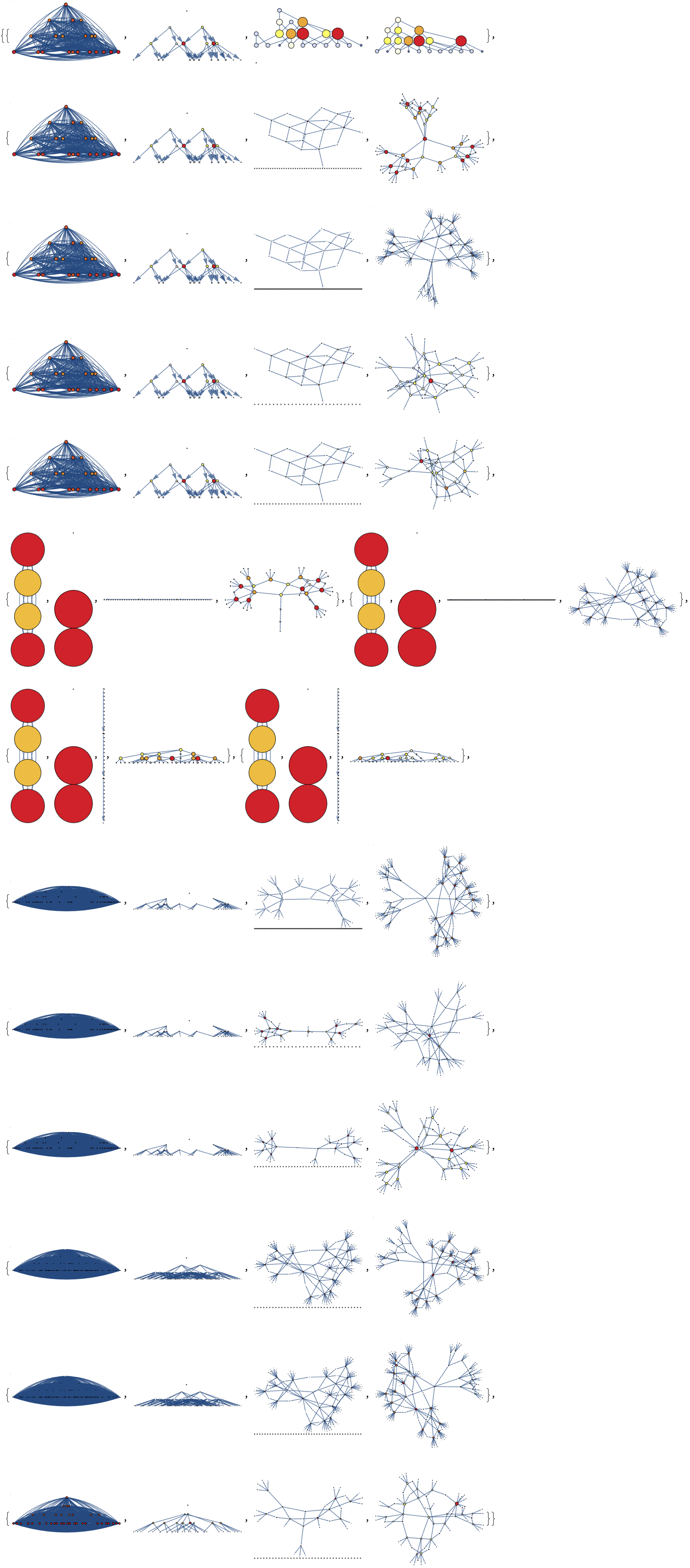
I think that I have the desire to describe how, since the whitespace between these graphs will always be there, at least we do know that can be removed, as this spaceship lifts off. Perhaps exploring and analyzing some edge cases in unison might make the behavior, quantum limitations, and multi-way dynamics of these tag systems more amazing. How?
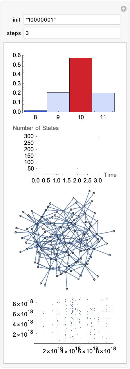
Manipulate[Column[{
   Module[{rulesGraph =
      ResourceFunction["MultiwaySystem"][{"00" -> "011", "10" -> "10",
         "01" -> "011", "11" -> "10"},
       init, steps, "StatesGraph"], rules},
    rules = List @@@ EdgeList[rulesGraph];
    Histogram[StringLength /@ Flatten[rules], {1}, "Probability",
     ColorFunction -> "TemperatureMap"]],
   Module[{rulesEvolution =
      ResourceFunction["MultiwaySystem"][{"00" -> "011", "10" -> "10",
         "01" -> "011", "11" -> "10"},
       init, steps, "AllEventsList"], numStates},
    numStates = Length /@ rulesEvolution;
    ListPlot[numStates, AxesLabel -> {"Time", "Number of States"}]],
   Module[{rulesGraph =
      ResourceFunction["MultiwaySystem"][{"00" -> "011", "10" -> "10",
         "01" -> "011", "11" -> "10"},
       init, steps, "StatesGraph"], rules},
    rules = List @@@ EdgeList[rulesGraph];
    Graph[DirectedEdge @@@ rules]],
   Module[{rulesGraph =
      ResourceFunction["MultiwaySystem"][{"00" -> "011", "10" -> "10",
         "01" -> "011", "11" -> "10"},
       init, steps, "StatesGraph"], rules},
    rules = List @@@ EdgeList[rulesGraph];
    ListPlot[Map[Hash, rules, {2}]]]}],
 {{init, "10000001", "init"}, ControlType -> InputField},
 {{steps, 3, "steps"}, ControlType -> InputField}]
It's already pre-processed. Does the post-processing have an effect? No. The interpretation of occurrences of specific patterns, and identifying patterns that can be represented more concisely, to make some analysis it is the most mechanistically pleasing way.
References
https://en.wikipedia.org/wiki/Emil_Leon_Post


