Message Boards Message Boards

0
|
1623 Views
|
7 Replies
|
7 Total Likes
View groups...
Share
Share this post:

Two spatial parametric curves merging with "acute angle"

Posted 1 year ago

Two spatial parametric curves of the fifth degree are given (the formulas are in the notebook attached. They have a common intersection point (for the first curve v = 1, for the second curve v = 0). As you can see on the graph, they seem to form an acute angle. What mathematical "indicator" says that the curves will "merge" exactly like this? I will immediately make a reservation that the derivatives of the first and second order of these curves are equal to each other at a common point.

POSTED BY: Aleksandr Miller
7 Replies

The lfirst curve "almost" turns 180 degrees not far from the point where it crosses the second curve:

a1[v_] = {1072 - 173.64999999999964` v - 1053.510000000002` v^2 - 
    4794.608388545948` v^3 + 10250.579098091992` v^4 - 
    4882.862709546044` v^5, -2579 + 367.7999999999993` v + 
    1085.800000000003` v^2 + 1474.5933742968045` v^3 - 
    4803.408260125245` v^4 + 2456.944885828447` v^5, 
   9.88383` + 643.53585` v - 560.0617000000002` v^2 - 
    604.8447774764995` v^3 + 817.3174429750306` v^4 - 
    192.31364549852992` v^5};
Minimize[a1'[v] . a1'[v], v]
ParametricPlot3D[
 a1[v], {v, (0.9846202694130824`) - .005, (0.9846202694130824`) + \
.005}, PlotStyle -> Red, PlotRange -> All]
POSTED BY: Gianluca Gorni

If the yellow and the blue curve were of the same function we could say that the function is not differentiable in this point, but there are two separate functions…

POSTED BY: Aleksandr Miller

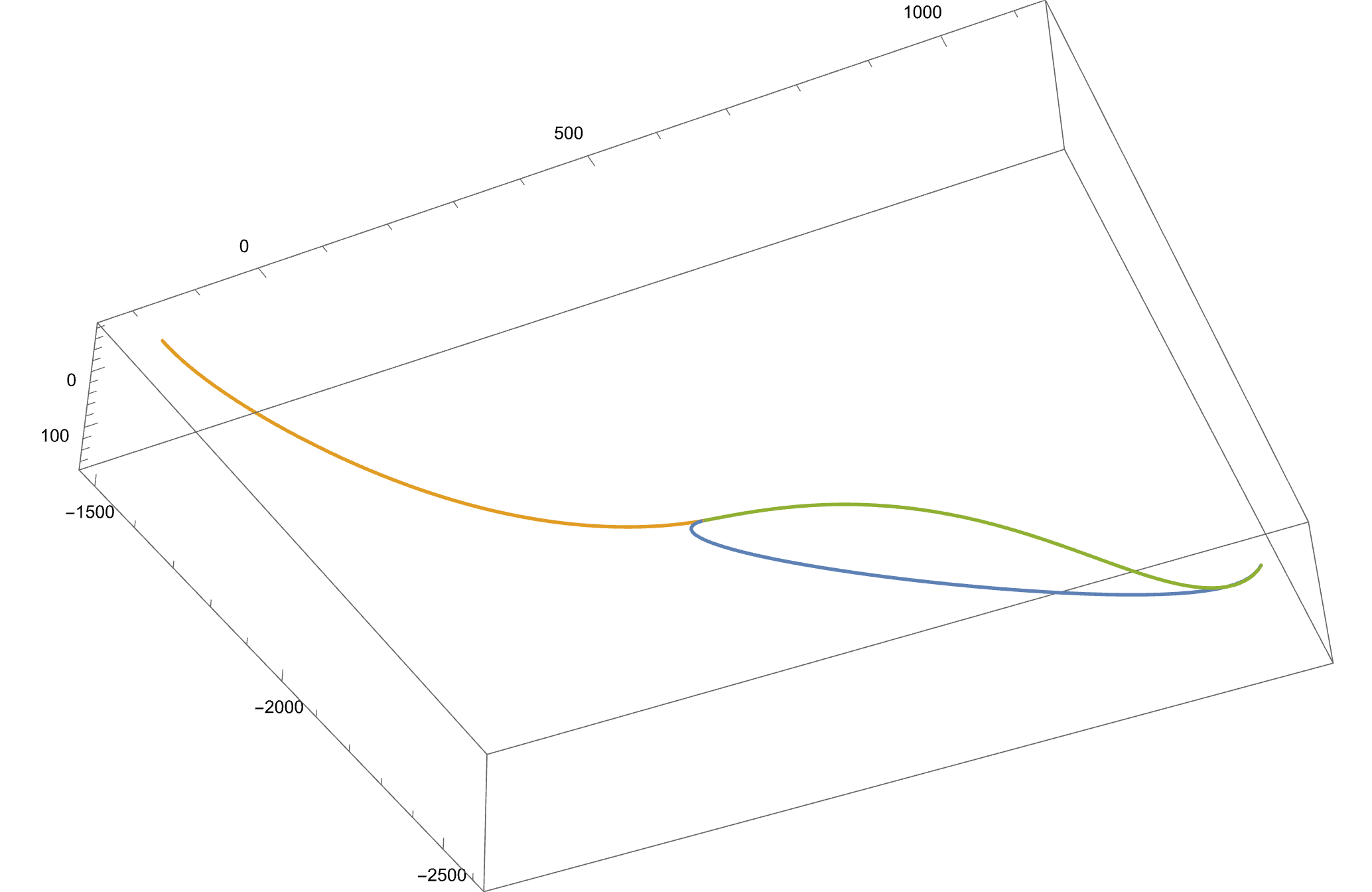
In fact, the most important question is how to determine that two curves at a common point will merge at such an "acute angle". I just don't know how to call it mathematically correct, so I use this term. I have attached a graph of three curves, of which the yellow and blue curve form an "acute angle", and the yellow and green do not form such an "angle". In fact, the angle between the tangents at a common point is 0 for both cases. But is there a way to determine without looking at the graph that the yellow curve "transitions" to the green one "smoothly", and to the blue one with a "peak". The equations of the curves: the blue curve: ,

\[Alpha] = {1072 - 173.64999999999964` v - 1053.510000000002` v^2 - 
   4794.608388545948` v^3 + 10250.579098091992` v^4 - 
   4882.862709546044` v^5, -2579 + 367.7999999999993` v + 
   1085.800000000003` v^2 + 1474.5933742968045` v^3 - 
   4803.408260125245` v^4 + 2456.944885828447` v^5, 
  9.88383` + 643.53585` v - 560.0617000000002` v^2 - 
   604.8447774764995` v^3 + 817.3174429750306` v^4 - 
   192.31364549852992` v^5}

, the yellow curve:

[Beta] = {417.948- 578.4099999999996 v - 243.95000000000118v^2 + 393.08600000000206 v^3 - 296.9425000000008v^4 + 121.26850000000013 v^5, -1997.27+ 259.14999999999964 v + 1303.1000000000022v^2 - 2037.5 v^3 + 1427.8500000000058v^4 - 475.4899999999998 v^5, 113.517+ 125.37 v + 476.27v^2 - 2032.92 v^3 + 1893.0629999999996v^4 - 652.1182 v^5}

, the green curve :

[Gamma] = {1072 - 173.64999999999964v - 1053.510000000002 v^2 + 2103.8958575598153v^3 - 3136.883524725092 v^4 + 1606.0956671652757v^5, -2579 + 367.7999999999993 v + 1085.800000000003v^2 - 794.1323873673391 v^3 - 449.44909006839225v^4 + 371.7114774357324 v^5, 9.88383+ 643.53585 v - 560.0617000000002v^2 - 1808.5353536247153 v^3 + 3135.9297882918345v^4 - 1307.2354146671187 v^5}

.I apologize in advance for the abundance of quotation marks and my own terms.enter image description here

POSTED BY: Aleksandr Miller

Here is a better view of the "merging" of the two curves:

a1[v_] = {1072 - 173.64999999999964` v - 1053.510000000002` v^2 - 
    4794.608388545948` v^3 + 10250.579098091992` v^4 - 
    4882.862709546044` v^5, -2579 + 367.7999999999993` v + 
    1085.800000000003` v^2 + 1474.5933742968045` v^3 - 
    4803.408260125245` v^4 + 2456.944885828447` v^5, 
   9.88383` + 643.53585` v - 560.0617000000002` v^2 - 
    604.8447774764995` v^3 + 817.3174429750306` v^4 - 
    192.31364549852992` v^5};
a2[v_] = {417.948` - 578.4099999999996` v - 243.95000000000118` v^2 + 
    393.08600000000206` v^3 - 296.9425000000008` v^4 + 
    121.26850000000013` v^5, -1997.27` + 259.14999999999964` v + 
    1303.1000000000022` v^2 - 2037.5` v^3 + 1427.8500000000058` v^4 - 
    475.4899999999998` v^5, 
   113.517` + 125.37` v + 476.27` v^2 - 2032.92` v^3 + 
    1893.0629999999996` v^4 - 652.1182` v^5};
sol13 = Solve[a1[v][[{1, 3}]] == a2[u][[{1, 3}]], {v, u}, Reals]
a1[v] == a2[u] /. sol13
sol13[[2]]
a1[v] == a2[u] /. sol13[[2]]
a1[1.000005220706588`] == a2[6.905467506898152`*^-7]
Show[ParametricPlot3D[
  a1[v], {v, (1.000005220706588`) - .2, (1.000005220706588`) + .1}, 
  PlotStyle -> Red, PlotRange -> All], 
 ParametricPlot3D[
  a2[u], {u, (6.905467506898152`*^-7) - .1, (6.905467506898152`*^-7) \
+ .1}],
 Graphics3D[{PointSize[.03], Red, Point[a1[(1.000005220706588`)]], 
   PointSize[.04], Opacity[.5], Black, 
   Point[a2[(6.905467506898152`*^-7)]]}]]
POSTED BY: Gianluca Gorni

What mathematical "indicator" says that the curves will "merge" exactly like this?

I would say it it the direction of the "velocity" vector. So - what is wrong with this most obvious approach?

v1 = Normalize[D[a1, v] /. v -> 1];
v2 = Normalize[D[a2, v] /. v -> 0];
Chop[v1 - v2]
(*  Out:   {0,0,0}  *)
POSTED BY: Henrik Schachner

Thanks a lot!

POSTED BY: Aleksandr Miller

Here is a calculation:

a1[v_] = {1072 - 173.64999999999964` v - 1053.510000000002` v^2 - 
    4794.608388545948` v^3 + 10250.579098091992` v^4 - 
    4882.862709546044` v^5, -2579 + 367.7999999999993` v + 
    1085.800000000003` v^2 + 1474.5933742968045` v^3 - 
    4803.408260125245` v^4 + 2456.944885828447` v^5, 
   9.88383` + 643.53585` v - 560.0617000000002` v^2 - 
    604.8447774764995` v^3 + 817.3174429750306` v^4 - 
    192.31364549852992` v^5};
a2[v_] = {417.948` - 578.4099999999996` v - 243.95000000000118` v^2 + 
    393.08600000000206` v^3 - 296.9425000000008` v^4 + 
    121.26850000000013` v^5, -1997.27` + 259.14999999999964` v + 
    1303.1000000000022` v^2 - 2037.5` v^3 + 1427.8500000000058` v^4 - 
    475.4899999999998` v^5, 
   113.517` + 125.37` v + 476.27` v^2 - 2032.92` v^3 + 
    1893.0629999999996` v^4 - 652.1182` v^5};
sol13 = Solve[a1[v][[{1, 3}]] == a2[u][[{1, 3}]], {v, u}, Reals]
a1[v] == a2[u] /. sol13
sol13[[2]]
a1[v] == a2[u] /. sol13[[2]]
a1[1.000005220706588`] == a2[6.905467506898152`*^-7]
Show[ParametricPlot3D[
  a1[v], {v, (1.000005220706588`) - .1, (1.000005220706588`) + .1}, 
  PlotStyle -> Red, PlotRange -> All], 
 ParametricPlot3D[
  a2[u], {u, (6.905467506898152`*^-7) - .1, (6.905467506898152`*^-7) \
+ .1}],
 Graphics3D[{PointSize[.03], Red, Point[a1[(1.000005220706588`)]], 
   PointSize[.04], Opacity[.5], Black, 
   Point[a2[(6.905467506898152`*^-7)]]}]]
VectorAngle[a1'[1.000005220706588`], a2'[6.905467506898152`*^-7]]
POSTED BY: Gianluca Gorni
Reply to this discussion
Community posts can be styled and formatted using the Markdown syntax.
Reply Preview
Attachments
Remove
or Discard

Group Abstract Group Abstract