Dear Sandu,
it's not MMA 10. MMA9 gives 5.96577, too. I cannot get the 1.42269 from that Youtube video in either MMA9 nor MMA10. I also do not get the warning shown in the Youtube video. I also cannot find a mistake in the equation.
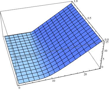
The 3D plot
Plot3D[V[S, t] /. sol, {S, 0.1, 25}, {t, 0, 1}]
also looks quite different from what it should look. More confusingly, in order to get the 3D plot of the video, I have to solve this differential equation:
sol = NDSolve[{D[V[S, t], t] + r*S*D[V[S, t], S]^2 +
     0.5 sigma*sigma* S ^2*D[V[S, t], {S, 2}] - r *V[S, t] == 0,
   V[S, T] == Max[S - K, 0], V[1000, t] == 1000 - K, V[0, t] == 0},
  V, {S, 0.1, 1000}, {t, 0, T}]
which has the derivative of the second term squared. I must be overlooking something, but I do not know what.
If I set the exponent of the S slightly larger than 1 it seems to work as well:
sol = NDSolve[{D[V[S, t], t] + r*S^1.04953 D[V[S, t], S] +
     0.5 sigma*sigma* S ^2*D[V[S, t], {S, 2}] - r *V[S, t] == 0,
   V[S, T] == Max[S - K, 0], V[1000, t] == 1000 - K, V[0, t] == 0},
  V, {S, 0.1, 1000}, {t, 0, T}]
There is a very sharp transition somewhere between 1.04952 and 1.04953. Okay. So this looks funny. I suppose that it has something to do with numerics. Let's try:
sol = NDSolve[{D[V[S, t], t] + r*S D[V[S, t], S] +
     0.5 sigma*sigma* S ^2*D[V[S, t], {S, 2}] - r *V[S, t] == 0,
   V[S, T] == Max[S - K, 0], V[1000, t] == 1000 - K, V[0, t] == 0},
  V, {S, 0.1, 1000}, {t, 0, T}, PrecisionGoal -> 10]
Now
V[S0, 0] /. sol
gives 1.42291. Success! The graph looks better, too:
Cheers,
Marco


