Here is some simple impl to draw the normal vector on a 2D function with rectangular support

Remove[bodeN]; (* bode normal *)
bodeN[fn_ (* function of two arguments *),
  {v1_, v10_, v11_} (* range of argument 1 *),
  {v2_, v20_, v21_} (* range of argument 2 *),
  l0_ (* length of normals *),
  p0_Integer: 20 (* plot points *)
  ] :=
 Module[{dv1, dv2, o, dfn1, dfn2, x, y, p, pp, pic0, pic1}, 
   (* Check fn *)
   If[FreeQ[fn[v1, v2], v1] || FreeQ[fn[v1, v2], v2], 
    Print["Function ", fn, " unabhaengig von ", v1, " und/oder ", 
     v2 "! Bye."];
    Return[$Failed]
    ];
   dv1 = (v11 - v10)/p0;
   dv2 = (v21 - v20)/p0;
   dfn1[x_, y_] := Evaluate[D[fn[x, y], x]];
   dfn2[x_, y_] := Evaluate[D[fn[x, y], y]];
   (* die Fusspunkte des Normalenfeldes - "in" der Flaeche *)
   p = Flatten[Table[{x, y, fn[x, y]}, {x, v10, v11, dv1}, {y, v20, v21, dv2}], 1];
   (* die Normalenrichtungen *)
   pp = (((l0/Sqrt[#.#]) & /@ #)*#) &[Flatten[Table[{dfn1[x, y], dfn2[x, y], -1}, 
       {x, v10, v11, dv1}, {y, v20, v21, dv2}], 1]];
   (* das l0 normierte Normalenrichtungsfeld mit Pfeilen *)
   pic1 = Graphics3D[{Arrowheads[.01], Arrow /@ Transpose[{p, p + pp}]}, DisplayFunction -> Identity];
   (* die Flaeche z = fn[v1, v2] selbst *)
   pic0 = Plot3D[fn[v1, v2], {v1, v10, v11}, {v2, v20, v21}, DisplayFunction -> Identity, PlotPoints->p0];
   (* Anzeige *)
   Show[{pic0, pic1}, DisplayFunction -> $DisplayFunction]
   ] /; l0 != 0 && v10 < v11 && v20 < v21 && AtomQ[v1] && 
   AtomQ[v2] && ! StringMatchQ[ToString[v1], ToString[v2]]

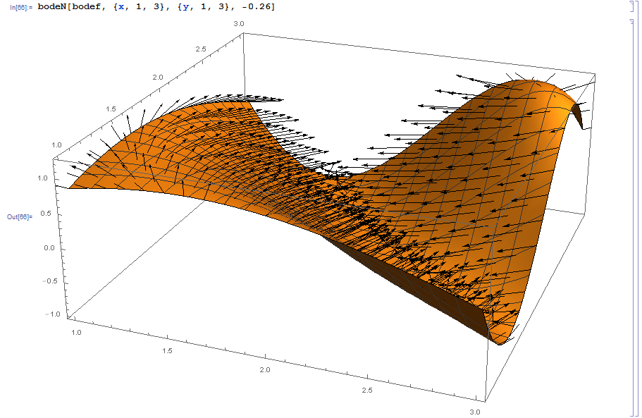
originating back from 2001; at that times there was a function ListPlotVectorField3D[] which has seemingly gone. bodeN gives Output like

Notebook attached.

Attachments:

Hi Marco,

That's quite useful.

I had not noticed that ListVectorPlot and ListVectorPlot3D are trying to re-interpolate the field and generate a plot on a regular grid. When I noticed that, I tried the option VectorPoints -> All, which is supposed to cause the vectors to be plotted only at the explicit points. That still did not work. I suppose that on a 2D manifold the interpolation algorithm is breaking down. This is too bad, since for a list plot I would really rather have a vector field plotted from an explicit list. I suppose I will make my own.

Best, David