Hi everyone. As I said in the previous discussion, I've started using Mathematica recently. I was assigned to solve a problem related to a simulation of a 2 DOF-quarter car model. Written the equations of motion (which corresponds to a system of coupled differential equations), I was able to solve for the position of the masses and then, by defining the functions that correspond to the solution of velocity and acceleration of the two bodies, I plotted the graphs for each solution and I guess that the problems responds with values of accelerations that are a little big (about 1000m/s^2). I'd like to ask your thoughts about it and eventually how can I solve the anomaly.

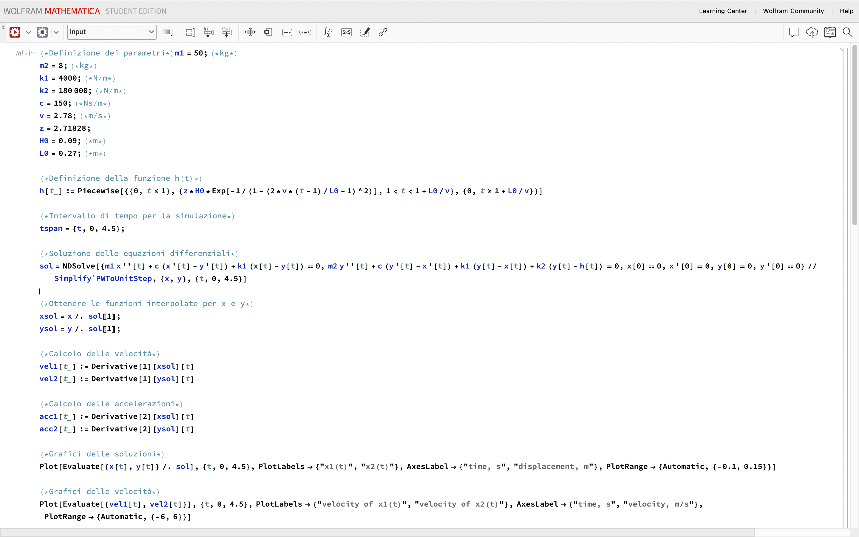
Here I'll write the code that I finalized for such solution, adding an image too, just to avoid ambiguity. In the last lines I'll talk about the context and Hyothesis that I am required to consider just to solve the problem.

m1 = 50; (*kg*)
m2 = 8; (*kg*)
k1 = 4000; (*N/m*)
k2 = 180000; (*N/m*)
c = 150; (*Ns/m*)
v = 2.78; (*m/s*)
z = 2.71828;
H0 = 0.09; (*m*)
L0 = 0.27; (*m*)


h[t_] := 
 Piecewise[{{0, t <= 1}, {z*H0*Exp[-1/(1 - (2*v*(t - 1)/L0 - 1)^2)], 
    1 < t < 1 + L0/v}, {0, t >= 1 + L0/v}}]

(*Intervallo di tempo per la simulazione*)
tspan = {t, 0, 4.5};


sol = NDSolve[{m1 x''[t] + c (x'[t] - y'[t]) + k1 (x[t] - y[t]) == 0, 
    m2 y''[t] + c (y'[t] - x'[t]) + k1 (y[t] - x[t]) + 
      k2 (y[t] - h[t]) == 0, x[0] == 0, x'[0] == 0, y[0] == 0, 
    y'[0] == 0} // Simplify`PWToUnitStep, {x, y}, {t, 0, 4.5}]


xsol = x /. sol[[1]];
ysol = y /. sol[[1]];


vel1[t_] := Derivative[1][xsol][t]
vel2[t_] := Derivative[1][ysol][t]


acc1[t_] := Derivative[2][xsol][t]
acc2[t_] := Derivative[2][ysol][t]


Plot[Evaluate[{x[t], y[t]} /. sol], {t, 0, 4.5}, 
 PlotLabels -> {"x1(t)", "x2(t)"}, 
 AxesLabel -> {"time, s", "displacement, m"}, 
 PlotRange -> {Automatic, {-0.1, 0.15}}]


Plot[Evaluate[{vel1[t], vel2[t]}], {t, 0, 4.5}, 
 PlotLabels -> {"velocity of x1(t)", "velocity of x2(t)"}, 
 AxesLabel -> {"time, s", "velocity, m/s"}, 
 PlotRange -> {Automatic, {-6, 6}}]


Plot[Evaluate[{acc1[t], acc2[t]}], {t, 0, 4.5}, 
 PlotLabels -> {"acceleration of x1(t)", "acceleration of x2(t)"}, 
 AxesLabel -> {"time, s", "acceleration, m/s^2"}, 
 PlotRange -> {Automatic, {-1000, 1000}}]

MATHEMATIC>

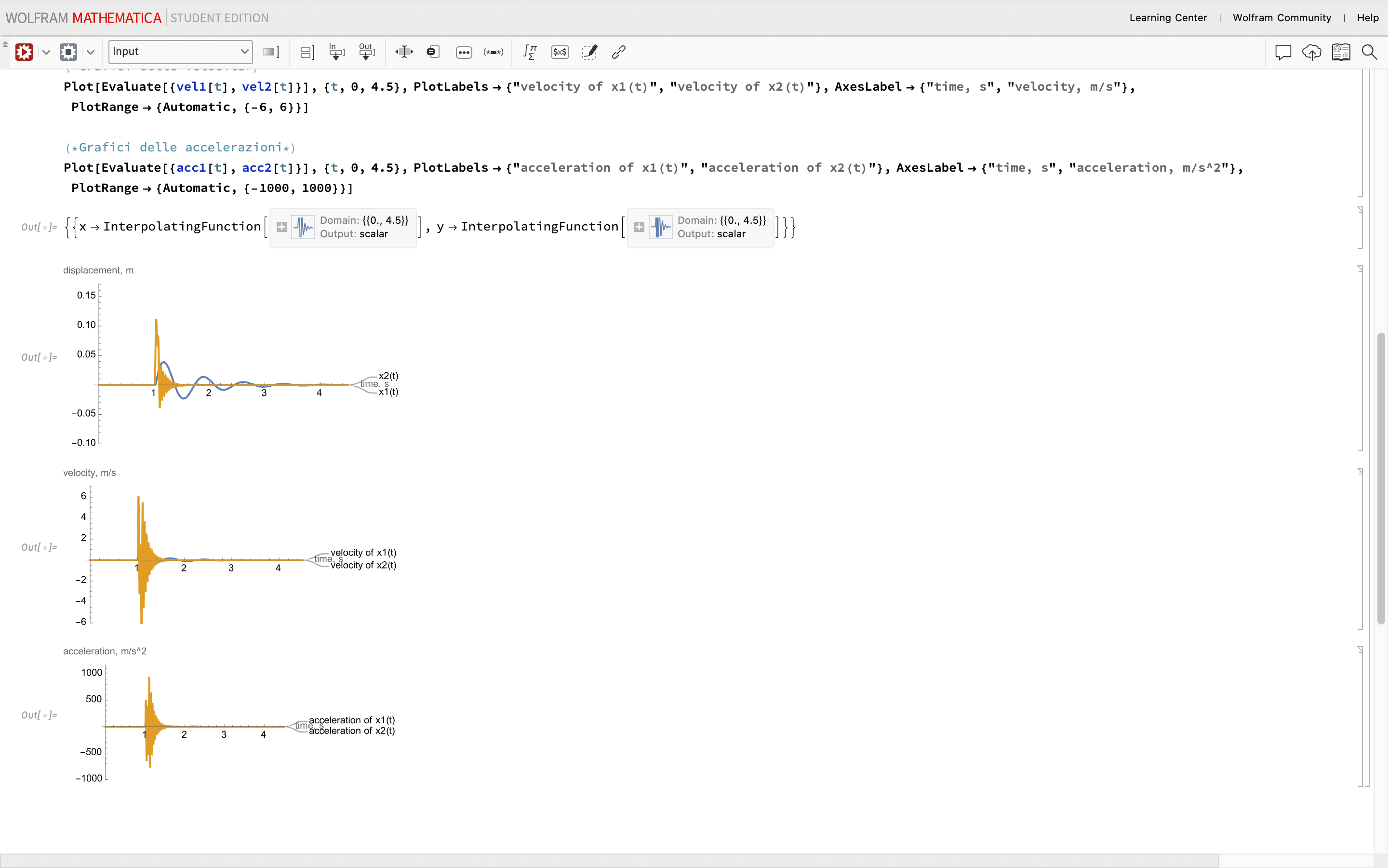
As you can see the last graphics shows values extremely high of accelerations and I am afraid to have inserted something incorrectly in the code.

For the context and the hypothesis of the problem, as I have previously anticipated it is about the simulation o fa quarter car model. The system is simplified as follows in the image below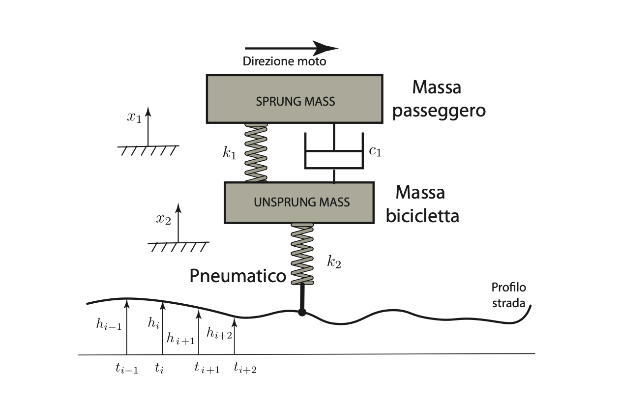

The Velocity of the system in the direction of motion is costant and so I can easily express the road profile in terms of time (and not space, as presented in the image below):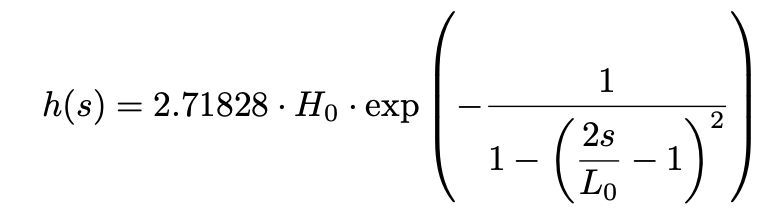

Furthermore the position x1(t) and x2(t) are calculated by the position of equilibrium of the respective mass. In conclusion the gravity force is not necessary.

I hope the context of the problem is clear. Can anyone explain me the error in the acceleration graphic?