Message Boards Message Boards

Plotting an expression where one of the parameters is satisfying a different equation

My question is very simple. I have a function $f(r)$ with some other parameters and I want to plot ${f'(r)}/{4\pi}$ vs P where r is satisfying the equation $f(r)=0$. I don't know where am I doing wrong. I have tried the following code but gives no answer. Can any one help me?

f[r_]:=1 - (a*Q^4)/(20*r^6) + Q^2/r^2 - (2*M)/r + (8/3)*P*Pi*r^2 - c*r^(-1 - 3*\[Omega]
Clear[a, c, \[Omega], Q, M]
a = 0.5; 
c = 0.2; 
\[Omega] = -3^(-1); 
Q = 0.7; 
M = 10; 
rH = r /. Solve[f[r] == 0, r, Reals];
Plot[D[f[r], r]/(4*Pi) /. r -> rH, {P, 0, 10}, PlotRange -> {0, 10}, PlotStyle -> Green, AxesOrigin -> {0, 0}]
POSTED BY: Debojyoti Mondal
7 Replies

Give a bounded interval for NSolve:

NSolve[f[r, P] == 0 && 10 > r > 0, r]
POSTED BY: Gianluca Gorni

I am following the same procedure for a different function here. But mathematica is not giving any result and shows some error. Is there something I am doing wrong here?

POSTED BY: Debojyoti Mondal
Posted 26 days ago

Ok, glad to hear it!

POSTED BY: Denis Ivanov

I get a plot with simply an Evaluate inside Plot:

f[r_] := 
  1 - (a*Q^4)/(20*r^6) + Q^2/r^2 - (2*M)/r + (8/3)*P*Pi*r^2 - 
   c*r^(-1 - 3*\[Omega]);
Clear[a, c, \[Omega], Q, M];
a = 0.5;
c = 0.2;
\[Omega] = -3^(-1);
Q = 0.7;
M = 10;
rH = r /. Solve[f[r] == 0, r, Reals];
Plot[Evaluate[D[f[r], r]/(4*Pi) /. r -> rH], {P, 0, 10}, 
 PlotRange -> {0, 10}, PlotStyle -> Green, AxesOrigin -> {0, 0}]
POSTED BY: Gianluca Gorni

Once again Thank you very much. I understood that they have used slightly different approach that is why the results are different. I got the exact graph.

POSTED BY: Debojyoti Mondal

First of all I Thank you very much. Yes, r is the radius and it is the largest positive root. So, I have used Last instead of First in the definition of fPlot in your code. I don't know why but Last command gives the largest positive root in my notebook and it worked nicely. Now to test this code, I have applied the same for published Article. You don't need to go through the full article but fig 3(a) is the desired result. I am getting almost similar graphs but slightly different. Am I still missing something? If you look at the last graph of fig 3(a) the range should be upto near 0.4 in y axis. But, i am getting upto 0.2.

POSTED BY: Debojyoti Mondal
Posted 27 days ago

First of all, you have some misprints. Please check if I fix them correctly.

 Clear[f, a, c, \[Omega], Q, M];
 a = 0.5;
c = 0.2;
\[Omega] = -3^(-1);
Q = 0.7;
M = 10;

f[r_, P_] := 
  1. - (a*Q^4)/(20*r^6) + Q^2/r^2 - (2*M)/r + (8/3)*P*Pi*r^2 - 
   c*r^(-1 - 3*\[Omega]);

Next, I strongly recommend using NSolve instead of Solve in this case.
Equation $f(r,P)=0$ has at least two solutions.

NSolve[f[r, 1.] == 0, r, Reals]
{{r -> -0.192412}, {r -> 1.30415}}

I guess r it's a radius, so we're going for the positive. But you can change that.
Finally, before plot a function it is desirable to define it separately.

Clear[fPlot];
fPlot[P_] := 
  D[f[r, P], r]/(4*Pi) /. 
   First@ NSolve[f[r, P] == 0 && r > 0, r, Reals];

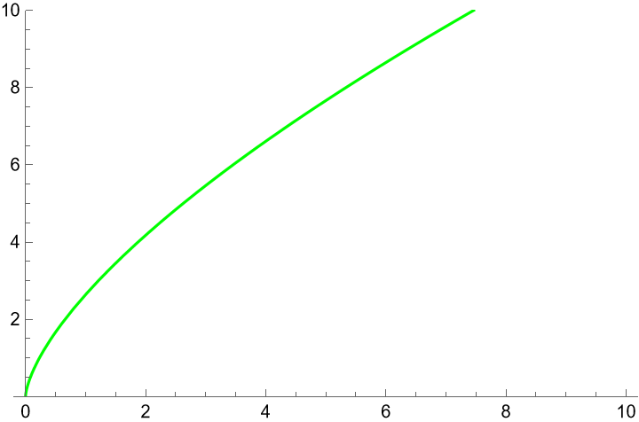
Plot[fPlot[P], {P, 0, 10}, PlotRange -> {0, 10}, PlotStyle -> Green, 
 AxesOrigin -> {0, 0}]

enter image description here

POSTED BY: Denis Ivanov
Reply to this discussion
Community posts can be styled and formatted using the Markdown syntax.
Reply Preview
Attachments
Remove
or Discard

Group Abstract Group Abstract