Message Boards Message Boards

0
|
1159 Views
|
9 Replies
|
0 Total Likes
View groups...
Share
Share this post:

Getting closed solution from Integrate or speeding up NIntegrate

I have a relatively complicated equation that needs to be integrated. Ideally I would like a closed-form solution, because I will use the solution over and over. How long should I wait for Mathematica (now Wolfram 14.1 for Mac) to "think" before I give it up as having no closed-form solution?

I have used NIntegrate, and it works, but it takes several hours to produce the 3D plot I need, and I need many of them. I have already taken as many approximations as I can afford; with the equation I have now, I will still be off by up to 1%, and I can't afford to be off by more.

I've never let Integrate run for 48 hours before, but I keep hoping it will come up with a solution.

Thanks, everyone who is interested! This is a simple laser propagation through a square aperture, but because I need to predict the output very close to the aperture I can't use the Fresnel approximation (it would be wrong by up to 30%). I'm using the full Huygens-Fresnel model but, since I am looking at a laser, the input is a plane wave.

POSTED BY: Russell Kurtz
9 Replies
Posted 5 months ago

A 3D plot can do tens of thousands, or many more, points and if each of those points requires a very slow calculation then that might partly explain why the plot is so slow.

If your function is sufficiently well behaved and the computer has some free time for an experiment, then you might try using Table to create a matrix of the values of your integral at specific points, using lots fewer points than your plot would otherwise default to. and do a ListPlot3D of that matrix. Experiment to see if you can find the number of points that will show the information you need to see and be faster than what you have now.

POSTED BY: Bill Nelson

FWIW, this returns unevaluated fairly quickly:

idx=0;
Integrate[insideParams4/.\[Eta]->y+\[Eta]/.Power[E,p_]:>E^Collect[foo=p,\[Eta],K[++idx]&],\[Eta]]

I've replaced the coefficients of η with generic parameters K[1], K[2],... and translated the integral η -> y + η. The relatively quick response indicates that Mathematica knows it cannot do this integral. However, it is not a definitive proof it cannot do your original integral. Your original integral might be a special case. But if there is no reason to think so, it probably is not.

If you want to continue trying to find an analytic integral, I'd suggest adding assumptions. For instance, I would guess that most or all of the variables and parameters are real. Integrate[] by default assumes they are complex.

POSTED BY: Michael Rogers

Thanks for the ideas. I am trying Assumptions; in the worst case I can try with numerical values for some of the variables. I did once take an integral that was solved after over 70,000 seconds (per AbsoluteTiming). It was also a little strange that the first time I ran this integration it gave me an error after 1716 seconds -- and the error was that I hadn't defined insideParams4.

I have found that making a table of values using ParallelTable, where I evaluated NIntegrate at 10,000 points, and it took significantly longer than using Plot3D. I haven't tried using Parallelize[NIntegrate]] because I have had many problems with that combination in the past.

The original integral has, for example, sqrt((xi-x)^2+(eta-y)^2+z^2). If I use a second-order approximation I get a closed-form solution but the integrand has errors of 10%. I might be able to accept 1%, which is why I'm trying this fourth-order approximation. I'm trying for a closed-form solution because calculating one for second order took about 1% as long as Plot3D on NIntegrate, and I was able to use Plot3D on a closed-form equation. But, as I said, second-order is not sufficient for this problem.

One thing I could also try is to compare the numerical integration time of the fourth-order approximation to that of the full equation using square roots. My instinct is that the square root would be equally fast or even faster, since the fourth-order version has three times as many variables.

Since I'm not a mathematician, I don't know much more than run this in Mathematica and see what happens. There are two standard approaches to this specific type of problem. One is the second-order approximation, which is insufficient for what I was trying to do; the other is limited to a size about 1/1000 of the area I need.

POSTED BY: Russell Kurtz
Posted 5 months ago

What range of parameters {x,y,z,w,lambda} are ?

Can you give a code to reproduce a 3D plot ?

POSTED BY: Updating Name

I'm trying to determine a general equation if possible. However, if we were to look at the actual value ranges, w will be between 100 and 250, x and y will be between -5w and +5w, z will be between w and 5000, and lambda will be between 0.5 and 1.5.

To make a 3D plot, first I would assign values to w, z, and lambda, something like

ts[x_,y_]:=testSquare/.{w->200,z->1000,lambda->1}

then plot as

Plot3D[ts[x,y],{x,-150,150},{y,-150,150}]

The integration over xi and nu would result in an equation in just x, y, z, w, and lambda. I did this using the second-order approximation and got accurate results for conditions that met the Fresnel diffraction requirements; here I'm looking for something where the second-order approximation results in errors exceeding 10%.

POSTED BY: Russell Kurtz

Regards M.I.

POSTED BY: Mariusz Iwaniuk

Change in the code to better resolution and better grid resolution:

   R = 2;(* If R parameter greater -grid resolution better,but the calculations take longer*)
   data0 = Outer[W0, Subdivide[-X, X, R*X], Subdivide[-Y, Y, R*Y]]; // AbsoluteTiming // First

The code is not mine, so for more information about it, please contact the creator Henrik Schumacher

POSTED BY: Mariusz Iwaniuk

Here's a slight refactoring of the code Mariusz adapted from Henrik that takes advantage of vectorization of math functions on my Mac M1. There is similar vectorization on Intel machines, but I cannot test them. Performance may vary. The vectorized functions evaluate vectors of input in parallel taking advantage of special CPU instructions (google SIMD). These usually evaluate large vectors of input more efficiently than a listable, parallelizable compiled function in Mathematica. However, the evaluation environment can get muddied by vectorized and nonvectorized operations, so that it is not always the case that a partially vectorized function will beat out a compiled function. In this case, I think it does for testSquare[]. I'll demonstrate the Gauss-Kronrod rule, because I can use it to estimate the error. One could also estimate the error in the Gauss rule by running it again with a different order and subtracting. The higher order rule generally has an error less than the difference, when the function has smooth derivatives up to the order of the rule.

I used Russell's initial formula to do a little optimization.

Clear[x, y, w, z, \[Lambda], \[Xi], \[Eta]]

z Exp[I 2 \[Pi] (
     x^4 (-15 y^4 + 12 y^2 z^2 - 8 z^4) + 
      8 z^4 (-y^4 + 4 y^2 z^2 + 8 z^4) + 
      4 x^2 (3 y^4 z^2 - 4 y^2 z^4 + 8 z^6))/(
     64 z^7 \[Lambda])]/(x^2 + y^2 + z^2) /. {x -> x1, y -> y1, 
  x^2 -> x2, x^4 -> x2^2, y^2 -> y2, y^4 -> y2^2(*,z^2->z2,z^4->z4,
  z^6->z6,z^7->z7*)}
(*
(E^((I \[Pi] (x2^2 (-15 y2^2 + 12 y2 z^2 - 8 z^4) + 
    8 z^4 (-y2^2 + 4 y2 z^2 + 8 z^4) + 
    4 x2 (3 y2^2 z^2 - 4 y2 z^4 + 8 z^6)))/(
 32 z^7 \[Lambda])) z)/(x2 + y2 + z^2)
*)

Here's is the optimized function. Subtract[a, b] and Divide[a, b] are usually available in vectorized forms. In normal Mathematica input and evaluation, when the arguments are not numbers or numeric arrays, they automatically change to Plus[a, Times[-1, b]] and Times[a, Power[b, -1]], respectively, which are somewhat less efficient. In Henrick's Outer[] code, the function is called with all input numeric or numeric arrays, so the efficient version of the arithmetic will be done. We will also make one other improvement. Instead of called testSquare[] twice, one for Re[] and once for Im[], we will call it and save the complex values. We can extract the real and imaginary parts later. (Sorry for all the details.)

testSquareG = Function[{x, y, w, z, \[Lambda], \[Xi], \[Eta]},
   With[{x2 = Subtract[x, \[Xi]]^2, y2 = Subtract[y, \[Eta]]^2},
    Divide[z, x2 + y2 + z^2] Exp[I \[Pi] *
       Divide[
        (x2^2 (-15 y2^2 + (12 z^2) y2 - 8 z^4) + 
          8 z^4 (-y2^2 + (4 z^2) y2 + 8 z^4) + 
          4 x2 ((3 z^2) y2^2 + (-4 z^4) y2 + 8 z^6)),
        32 z^7 \[Lambda]]
      ]
    ]
   ];

{pts, weights, errweights} = (* this is the same except for the Rule *)
  NIntegrate`GaussKronrodRuleData[5, MachinePrecision];
m = 20;(*If the m parameter is greater,than is better resolution*)
n = 20;(*If the n parameter is greater,than is better resolution*)
w = 200.;(* w = 200 *)
z = 1000.;(* z = 1000 *)
\[Lambda] = 1.;(* \[Lambda] = 1 *)
\[Xi]data = Partition[Subdivide[-w/2, w/2, m], 2, 1];
\[Eta]data = Partition[Subdivide[-w/2, w/2, n], 2, 1];
{\[Xi], \[Eta]} = Transpose[
   Tuples[{Flatten[\[Xi]data . {1. - pts, pts}], 
     Flatten[\[Eta]data . {1. - pts, pts}]}]];
\[Omega] = Flatten[KroneckerProduct[
    Flatten[KroneckerProduct[Differences /@ \[Xi]data, weights]], 
    Flatten[KroneckerProduct[Differences /@ \[Eta]data, weights]]]];
\[Epsilon] = Flatten[KroneckerProduct[ (* for estimating error *)
    Flatten[KroneckerProduct[Differences /@ \[Xi]data, errweights]], 
    Flatten[KroneckerProduct[Differences /@ \[Eta]data, errweights]]]];

WW = {x, y} |-> {x, y, (* complex values of  testSquareG function !!! *)
  testSquareG[x, y, w, z, \[Lambda], \[Xi], \[Eta]] . \[Omega]};
X = 150.;(*Range for: X\[Element](-150,150) *)
Y = 150.;(*Range for: Y\[Element](-150,150) *)
dataC = Outer[WW, Subdivide[-X, X, 100], Subdivide[-Y, Y, 100]]; // 
  AbsoluteTiming // First

ListPlot3D[Flatten[Re@dataC, 1], PlotRange -> All, 
 AxesLabel -> {"x", "y", "Z"}, ColorFunction -> "Topographic", 
 PlotLabels -> HoldForm[Re[testSquareG[x, y]]]]
ListPlot3D[Flatten[MapAt[Im, dataC, {All, All, 3}], 1], 
 PlotRange -> All, AxesLabel -> {"x", "y", "Z"}, 
 ColorFunction -> "Topographic", 
 PlotLabels -> HoldForm[Im[testSquareG[x, y]]]]

The plots are similar to Mariusz's. With the Gauss-KronrodRule, we can examine the error estimate:

errWW = {x, y} |-> testSquareG[x, y, w, 
     z, \[Lambda], \[Xi], \[Eta]] . \[Epsilon]; (* GK error estimates *)
X = 150.;(*Range for: X\[Element](-150,150) *)
Y = 150.;(*Range for: Y\[Element](-150,150) *)
err = Outer[errWW, Subdivide[-X, X, 100], Subdivide[-Y, Y, 100]]; // 
  AbsoluteTiming // First

(*  15.093  *)

err // Flatten // RealExponent // 
 ListPlot[#, PlotLabel -> Element[HoldForm@Log10@Abs[err], MinMax[#]]] &
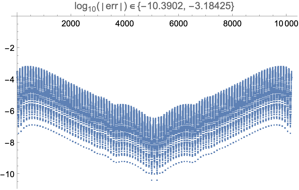
error plot between 10^-10 and 10^-3

If we increase the order to NIntegrate`GaussKronrodRuleData[7, MachinePrecision], it takes 25 sec. instead of 15, and the error drops to between 10^-14 and 10^-7.


Addendum

FWIW, we can mimic Mariusz's and Henrik's approach with NIntegrate[] as follows It won't be nearly as fast as the raw integration code (it takes 100 sec., half the time Mariusz's NIntegrate[] mathod takes on my Mac). However, it may be easier to understand.

testSquareF[x_?NumericQ, y_?NumericQ, w_?NumericQ, z_?NumericQ, \[Lambda]_?NumericQ] := 
  NIntegrate[(E^((I \[Pi] (8 z^4 (8 z^4 + 
          4 z^2 (y - \[Eta])^2 - (y - \[Eta])^4) + 
       4 (8 z^6 - 4 z^4 (y - \[Eta])^2 + 
          3 z^2 (y - \[Eta])^4) (x - \[Xi])^2 + (-8 z^4 + 
          12 z^2 (y - \[Eta])^2 - 15 (y - \[Eta])^4) (x - \[Xi])^4))/(
    32 z^7 \[Lambda])) z)/(
   z^2 + (-y + \[Eta])^2 + (-x + \[Xi])^2), {\[Xi], -w/2, 
    w/2}, {\[Eta], -w/2, w/2}, PrecisionGoal -> 4, MinRecursion -> 4, 
   MaxRecursion -> 4, Method -> {"GaussKronrodRule", "Points" -> 7}];

With[{n = 4(*If the n parameter is smaller, than is better resolution*)}, 
  ListPlot3D[
   Partition[
    Flatten[ParallelTable[{x, y, 
       Re[testSquareF[x, y, 200, 1000, 1]]}, {x, -150, 150, 
       n}, {y, -150, 150, n}, Method -> "FinestGrained"]], 3], 
   ColorFunction -> "Topographic", 
   PlotLabels -> HoldForm[Re[testSquareF[x, y]]]]] // AbsoluteTiming

(* picture like Mariusz's *)
POSTED BY: Michael Rogers

Wow, I'm learning so much about speeding up plotting here...This version took 16.8 seconds to run on my computer, the previous best was nearly 150 seconds and my original was almost 400 seconds. At 16.8 seconds it isn't worth it any more to try to find a closed-form solution.

Thanks!

POSTED BY: Russell Kurtz
Reply to this discussion
Community posts can be styled and formatted using the Markdown syntax.
Reply Preview
Attachments
Remove
or Discard

Group Abstract Group Abstract