You're using the discrete Fourier transform and the whole split-operator method thing to solve the two-dimensional Schrödinger equation. In the first code block, the wave packet with momentum primarily in the y-direction, is splitting into two parts after a few time steps. Is this physically correct for a free particle? I think the error is not an intrinsic issue of splitting wave packets, but the potential issue lies with numerical resolution or accuracy.

TDFourier2D[timesteps_, potheight_, ellip_] := 
 Module[{NP, L, dx, dt, kx, ky, x0, y0, xmax, xmin, ymax, ymin, kxmax,
    kymax, \[Rho], TimeEnd, psi, K3, nt, UK, UV, kgridx, kgridy}, 
  NP = 100; L = 1; dx = L/(NP - 1); dt = (1/20)  dx^2; 
  TimeEnd = timesteps; \[Rho] = 0.16; x0 = 0.0; y0 = 0.0; kx = 0; 
  ky = 50; xmax = 1; xmin = -1; ymax = 1; ymin = -1; 
  kgridx = Array[# &, {NP}, {-Pi/dx, Pi/dx}];
  kgridy = Array[# &, {NP}, {-Pi/dx, Pi/dx}];
  psi3[0] = 
   Array[(1/(\[Rho]  Sqrt[
            Pi]))  Exp[-I  kx  #1 - (#1 - x0)^2/(2  \[Rho]^2)]*
       Exp[-I  ky  #2 - (#2 - y0)^2/(2  \[Rho]^2)] &, {NP, 
      NP}, {{xmin, xmax}, {ymin, ymax}}] // Quiet;
  K3 = 1/2  (kgridx^2 + kgridy^2);
  V3 = Array[(potheight/2)  #1^2 + (ellip*potheight/2)  #2^2 &, {NP, 
     NP}, {{xmin, xmax}, {ymin, ymax}}];
  UV[dt_] := Exp[-I  V3  dt];
  UK[dt_] := Exp[-I  K3  dt];
  U[dt_]@psi_ := UV[dt]*InverseFourier[UK[dt]*Fourier[psi]];
  Do[psi3[nt] = U[dt][psi3[nt - 1]], {nt, 1, TimeEnd}];
  psi3]
ellipticalform = 0.2; 
TimeEnd = 160; 
potheight = 0; 
{timing, psi3Result} = 
  AbsoluteTiming[TDFourier2D[TimeEnd, potheight, ellipticalform]];
graphTable1 = 
 GraphicsGrid[
  Partition[
   Table[Labeled[
     ListDensityPlot[Abs[psi3Result[i]], Axes -> True, 
      PlotRange -> All, ColorFunction -> "SunsetColors", 
      PerformanceGoal -> "Quality"], {"x", "y"}, {Left, Top}, 
     RotateLabel -> True], {i, 1, TimeEnd, TimeEnd/4}], 2], 
  Frame -> All, ImageSize -> 400]

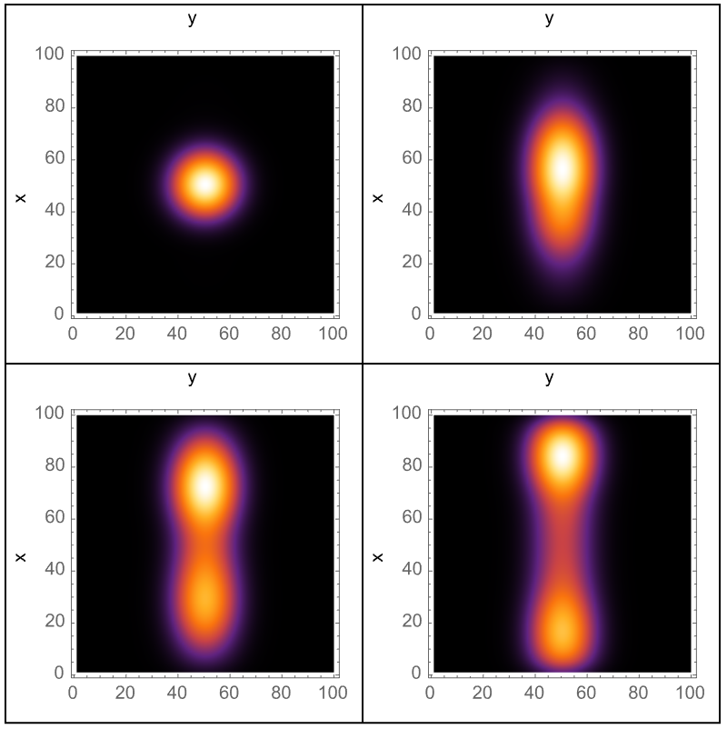
Now if I can just get my mouse working, I think that the importance of grid resolution and time step size is a critical way to accurately simulate the Schrödinger equation. It turns out that using the split-operator method, it's possible to increase the grid re-solution which therefore minimizes the effect, of aliasing in the Fourier transform. This might seem like something we could do by zooming in on the grid but no, we've got to clear out what we've got programmatically which will allow us to try a smaller time step. But you can try all the smaller time steps and when you do, you will find that the wave packet's evolution is accurately computed at each step, reducing the computational errors that could lead to the wave packet's artificial splitting. I imagine that in future versions of the Wolfram Language these Pandas-like artifacts such as splitting wherein a large dt might not capture the dynamics accurately, will never have a smaller dt that reduces these inaccuracies. In the following block of code you will discover that a smaller time step in fact does lead to more accurate time evolution, especially in this newfangled split-operator method, which relies on operator splitting over small intervals.

TDFourier2D[timesteps_, potheight_, ellip_] := 
 Module[{NP, L, dx, dt, kx, ky, x0, y0, xmax, xmin, ymax, ymin, kxmax,
    kymax, \[Rho], TimeEnd, psi, K3, nt, UK, UV, kgridx, kgridy}, 
  NP = 256; L = 1; dx = L/(NP - 1); dt = (1/50)  dx^2; 
  TimeEnd = timesteps; \[Rho] = 0.16; x0 = 0.0; y0 = 0.0; kx = 0; 
  ky = 50; xmax = 1; xmin = -1; ymax = 1; ymin = -1; 
  kgridx = Array[# &, {NP}, {-Pi/dx, Pi/dx}];
  kgridy = Array[# &, {NP}, {-Pi/dx, Pi/dx}];
  psi3[0] = 
   Array[(1/(\[Rho]  Sqrt[
            Pi]))  Exp[-I  kx  #1 - (#1 - x0)^2/(2  \[Rho]^2)]*
       Exp[-I  ky  #2 - (#2 - y0)^2/(2  \[Rho]^2)] &, {NP, 
      NP}, {{xmin, xmax}, {ymin, ymax}}] // Quiet;
  K3 = 1/2  (kgridx^2 + kgridy^2);
  V3 = Array[(potheight/2)  #1^2 + (ellip*potheight/2)  #2^2 &, {NP, 
     NP}, {{xmin, xmax}, {ymin, ymax}}];
  UV[dt_] := Exp[-I  V3  dt];
  UK[dt_] := Exp[-I  K3  dt];
  U[dt_]@psi_ := UV[dt]*InverseFourier[UK[dt]*Fourier[psi]];
  Do[psi3[nt] = U[dt][psi3[nt - 1]], {nt, 1, TimeEnd}];
  psi3]
ellipticalform = 0.2; 
TimeEnd = 160;
potheight = 0;
{timing, psi3Result} = 
  AbsoluteTiming[TDFourier2D[TimeEnd, potheight, ellipticalform]];
graphTable1 = 
 GraphicsGrid[
  Partition[
   Table[Labeled[
     ListDensityPlot[Abs[psi3Result[i]], Axes -> True, 
      PlotRange -> All, ColorFunction -> "SunsetColors", 
      PerformanceGoal -> "Quality"], {"x", "y"}, {Left, Top}, 
     RotateLabel -> True], {i, 1, TimeEnd, TimeEnd/4}], 2], 
  Frame -> All, ImageSize -> 400]

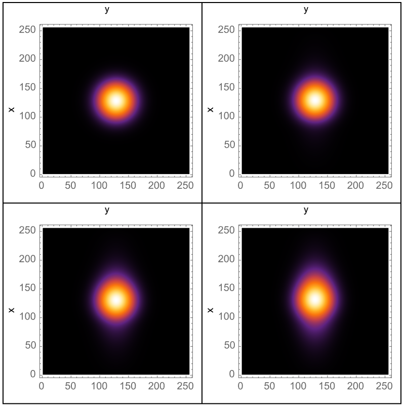
That is how we make sure that in this third iteration we have increased the grid resolution "NP". A higher grid resolution, means we use more points to represent the wave function, which improves the accuracy of the discrete Fourier transform and so on and so forth. This helps in reducing numerical artifacts such as aliasing, which is an implicit unintended splitting of the wave packet. And that is why yes, the wave packet with momentum primarily in the y-direction is splitting into two parts after a few time steps, which isn't physically correct for a free particle. This begs the question of whether we can articulate how we achieve all our..wave packets with regard to sufficient resolution to minimize aliasing effects and gauging smaller time steps such that the wave packet's evolution is continuously and accurately computed at each step.