Hello,

Thank you for your question. I noticed that the initial approach had some issues related to visibility and interpretation, which might be why the figure was not coming out as expected.

One issue was the presence of an "invisible" tooltip that would only appear when hovering over the points on the graph. That's the thing about plot colors, people usually leave the defaults. This made it difficult to see and interpret the color-coded graph correctly, as the key points (like the inversion point) were not immediately visible without interaction. Moreover, I didn't even want to answer this question right away because the default settings didn't make it clear what color values or sizes the points were using, adding to the confusion.

Here's the initial code I started with, tag strings and all:

Clear[pr, tm, r, M, Q, \[Alpha]]
pr[r_] := (8*Pi*M*r^2 - 3*Pi^2*\[Alpha]*r^2 - 3*Pi^2*r^4 - 4*Q^2)/(4*
     Pi^3*r^6);
tm[r_] := (16*Pi*M*r^2 - 6*Pi^2*\[Alpha]*r^2 - 3*Pi^2*r^4 - 
     12*Q^2)/(6*Pi^3*r^3*(2*\[Alpha] + r^2));
Q = Sqrt[3]*Pi;
M = 7;
\[Alpha] = 0.2;
points = Table[{pr[r], tm[r]}, {r, 0.01, 2, 0.02}];
point1 = {0, 0.055}; 
point2 = {0.1136, 0.1641};
point3 = {0.2, 0};
ParametricPlot[{{pr[r], tm[r]}}, {r, 0.01, 2}, 
 PlotRange -> {{0, 0.21}, {0, 0.2}}, AspectRatio -> 1, 
 PlotStyle -> Thick, 
 Epilog -> {Red, PointSize[Large], Point[point2], PointSize[Medium], 
   Black, Point /@ points, 
   Text[Style["(0.1136, 0.1641)", Black, 12], point2, {1, -1}]}, 
 AxesLabel -> {"P", "T"}]

If there's one thing I do know to address these issues it's that without explicitly setting the colors and sizes of points, it becomes unclear how these are being rendered, leading to possible mis-interpretation.

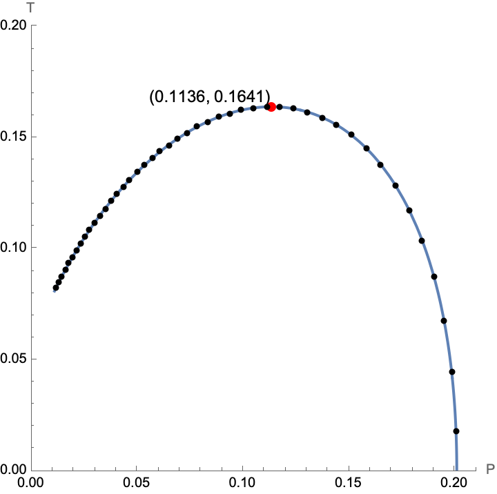
To address these issues, I modified the code to elaborate on how in the most immediate sense we could show the theoretical particles that do exist, you might have a chance with the points labeled directly on the plot using the Text function. This reminds me of those parameteric functions for describing axions. The answer is pretty subtle; label the points directly on the plot using the Text function, which makes it easier to identify the points and understand their significant in the illuminating context of the plot.