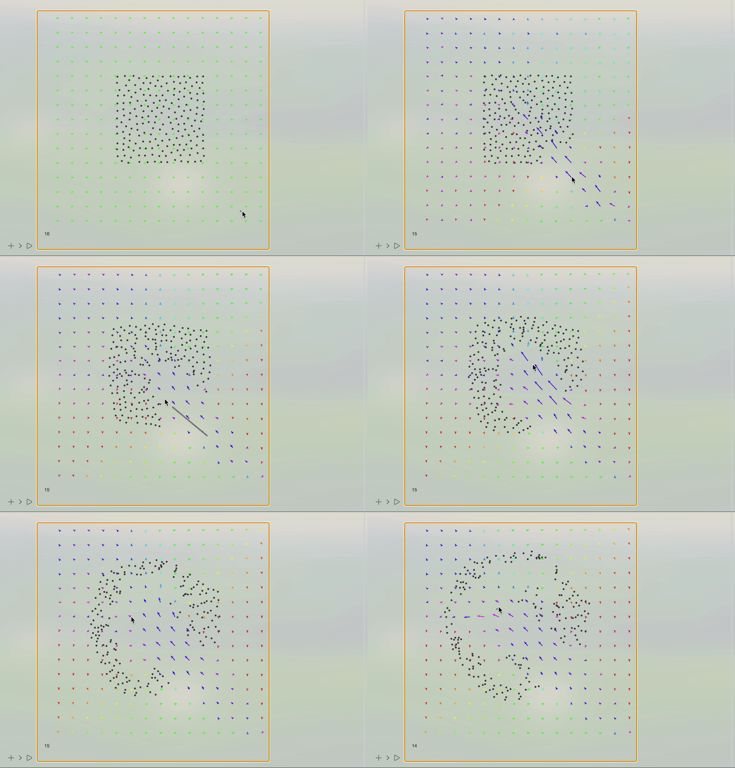
In this notebook, we will continue to explore a simple technique for simulating 2D incompressible fluids for visual effects. This work is mostly based on Jos Stam. Stable Fluids SIGGRAPH 1999 as well as a tutorial by Karl Sims
Advection
From mathematica point of view it describes a general process of moving something on a scalar or vector field in the direction given by another vector field.
For simplicity's sake, we will first start with scalar fields.
grid = Table[{0, 0}, {5}, {5}]; grid[[3, 3]] = {0, 1};
u = Table[1., {5}, {5}];(*our scalar field we will move*)
One can think about u as if it were a mass of something, which will be carried by the stream grid.
Naive approach
Looking at the borders 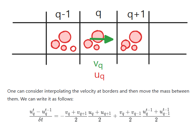
Warning: this is wrong
advect[v_, u_, \[Delta]t_ : 0.1] :=
 With[{max = Length[v]},
  With[{take =
     Function[{array, x, y},
      If[x >= 1 && x <= max && y >= 1 && y <= max, array[[x, y]],
       array[[1, 1]]  0.]]},
   Table[With[{v2 = ((take[v, i, j + 1] +
             take[v, i, j])/(2.0)) . {0, -1},
       v4 = (((take[v, i, j - 1] + take[v, i, j])/(2.0)) . {0, 1},
         org = u[[i, j]]},
      org + (v4  ((take[u, i, j - 1] + org)/(2.0)) +
          v2   ((take[u, i, j + 1] + org)/(2.0)))  \[Delta]t], {i,
      max}, {j, max}] // Chop]]
Now if we test it on our u field
u = Table[1., {5}, {5}];
Table[MatrixPlot[Nest[advect[grid, #] &, u, n],
ImageSize -> 200], {n, {0, 1, 100}}];
Riffle[%,
HTMLView["<span style=\"font-size:2.5rem\">→</span>"]] // Row
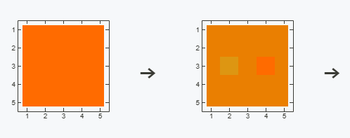
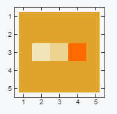
We can check it numerically as well
Nest[advect[grid, #] &, u, 100] // Chop // MatrixForm

or in a more creative way
Map[Function[cell, RGBColor[Tanh[cell], 0,-Tanh[cell]]], Nest[advect[grid, #]&, u, 100], {2}];
% // MatrixForm
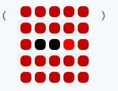
Now we are ready to apply this knowledge to our fluid simulation. But how?
Advection differential equation
I would like to draw your attention to the differential equation of advection

If one tries to descritize it on 1D grid 
After substituting it back, one finds, that it matches our previous equation we found for a problem of moving "mass" on a grid. ==We solved this exact differnetial advection equation while implementing advect function.==
Fluid Momentum
Newton's second law in the Navier-Stokes equation is defined by the following term.

Does it remind you anything?.. The conservation of momentum of our fluid is actual self advection.
To simulate fluid momentum, the flow field can simply flow itself. Flow vectors are updated by reading interpolated values from upstream grid cells in the same way the tracer image is advected above. New vector values are pulled from the negative direction of flow.
To test it, one can construct the same sandbox used in Part 1, but change the update loop slightly.
vgrid = Table[{0., 0.}, {i, 15}, {j, 15}];
     vcolors = Table[1.0, {Length[vgrid]}, {Length[vgrid]}];

     start = {1, 1};
     drawing = False;
     dest = {0, 0};
     vfps = 0;

     With[{win =
        CurrentWindow[],(*save the current window to append graphics*)
       currentCell = ResultCell[]},
      EventHandler[
       win, {"Closed" ->
         Function[Null,
          Delete[currentCell] (*remove output cell if a notebook has \
been closed*)(*this will prevent the animation running uncontrollably \
on the next start*)]}];
      Graphics[{Table[
          With[{i = i,
            j = j},(*now we have dynamic Hue and dynamic Arrow*)
           Offload[{Hue[vcolors[[i]][[j]]],
             Arrow[{{i, j}, {i, j} + vgrid[[i]][[j]]}]}]], {i,
           15}, {j,
           15}](*attach listeners to a user's mouse to manipulate the \
grid*) EventHandler[
          Graphics`Canvas[], {"mouseup" ->
            Function[xy,
             With[{v = -Normalize[start - xy]},
              Do[(*draw a line of velocities*)
                With[{p = Round /@ ((xy - start)  a + start)},
                  If[p[[1]] <= 15 && p[[1]] >= 1 && p[[2]] <= 15 &&
                    p[[2]] >= 1,
                    vgrid[[p[[1]], p[[2]]]] = {v[[1]],
                    v[[2]]};];];, {a, 0, 1, 0.1}];];
             Delete[drawing];(*delete temporal arrow*)
             drawing = False;],
           "mousemove" -> Function[xy, dest = xy;],
           "mousedown" -> Function[xy, start = xy;
             dest = xy;
             If[drawing =!= False, Delete[drawing]];
             (*BB[*)(*append GUI's arrow to existing canvas*)
             drawing =
              FrontSubmit[{AbsoluteThickness[3], Gray,
                Arrow[{xy, dest // Offload}]}, MetaMarker["vcanvas"],
               "Window" -> win,
               "Tracking" ->
                True (*enable tracking of created \
object*)];]}],(*sync with browser's repaint cycle and update of fps \
label*)AnimationFrameListener[vfps // Offload, "Event" -> "vframe"],
        (*mark this instance of Graphics with uid to append new \
elements*)
        MetaMarker["vcanvas"], Text[vfps // Offload, {0, 0}]},
       Controls -> False, ImageSize -> 500,
       PlotRange -> {{-0.5, 15.5}, {-0.5, 15.5}},
       ImagePadding -> None, TransitionType -> None]]

     (*subscribe to animation event*)

     vtime = AbsoluteTime[];

     EventHandler["vframe",
      Function[Null (vgrid = advect[vgrid, vgrid] // N);
       vcolors =
        Map[Function[
          val, ((\[Pi] + 2.0  ToPolarCoordinates[val] //
              Last) (/(3.0  \[Pi]))], vgrid, {2}];
   vfps = (((vfps + 1/(AbsoluteTime[] - vtime)))/(2.0)) // Round;
   vtime = AbsoluteTime[];]];
In the end it should be similar to what is shown on the animation 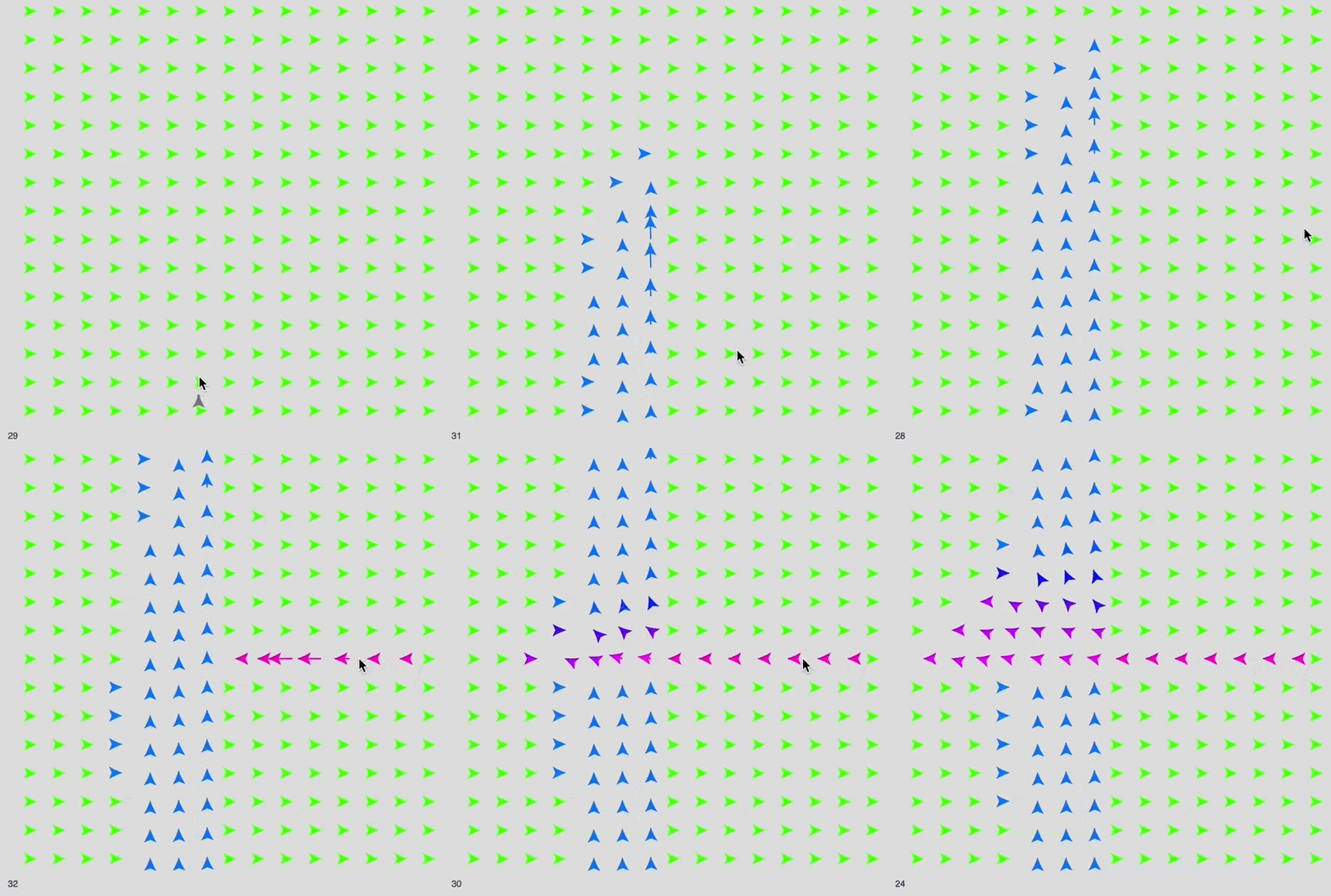
Test particles
In order to better visualize the fluid, we need something to be moved by our stream. The simplest solution is to spread hundreds of tracer particles. The velocity field can push them in the direction interpolated bilinearly from the grid.
Bilinear interpolation
This is the most basic thing to implement. This probably is not the fastest version, but good enough for educational purposes.
bilinearInterpolation[array_, {x0_, y0_}] :=
 Module[{rows, cols, x = y0, y = x0, x1, x2, y1, y2, fQ11, fQ12, fQ21,
    fQ22},(*Get the dimensions of the array*){rows, cols} =
   Take[Dimensions[array], 2];
  (*Clip points to the boundaries*)x = Clip[x, {1, cols}];
  y = Clip[y, {1, rows}];
  (*Find the bounding indices*)x1 = Floor[x];
  x2 = Ceiling[x];
  y1 = Floor[y];
  y2 = Ceiling[y];
  (*Get the values at the four corners*)fQ11 = array[[y1, x1]];
  fQ12 = array[[y2, x1]];
  fQ21 = array[[y1, x2]];
  fQ22 = array[[y2, x2]];
  (*Perform bilinear interpolation*)
  If[x2 == x1,
   If[y2 == y1, fQ11,
    1/(2  (y2 - y1))*(fQ11  (y2 - y) + fQ21  (y2 - y) +
       fQ12  (y - y1) + fQ22  (y - y1))],
   If[y2 == y1,
    1/(2  (x2 - x1))*(fQ11  (x2 - x) + fQ21  (x - x1) +
       fQ12  (x2 - x) + fQ22  (x - x1)),
    1/((x2 - x1)  (y2 - y1))*(fQ11  (x2 - x)  (y2 - y) +
       fQ21  (x - x1)  (y2 - y) + fQ12  (x2 - x)  (y - y1) +
       fQ22  (x - x1)  (y - y1))]]]
One can check if it works correctly by scaling up some raster images
bmp = Table[{Power[Cos[y], 2], Power[Sin[x], 2], 0.5} // N, {x, 0, Pi,
     Pi/5}, {y, 0, Pi, Pi/5}];
ibmp = Table[
   bilinearInterpolation[bmp, {x, y}], {x, 1, 6 - 0.1, 0.1}, {y, 1,
    6 - 0.1, 0.1}];

{Image[bmp, "Real32", Magnification -> 50, Antialiasing -> False],
  Image[ibmp, "Real32", Magnification -> 6]} // Row


On the right, there is our interpolated array, while on the left, the original one
Uniform distribution
There is another short problem to solve: how to distribute particles evenly over a defined region. However, there is a solution out of the box in the Wolfram Language standard library.
RandomPointConfiguration[HardcorePointProcess[10000, 0.4, 2],
    Rectangle[{1, 1}, {5, 5}], Method -> {"LengthOfRun" -> 10000000}][
   "Points"] // Point // Graphics
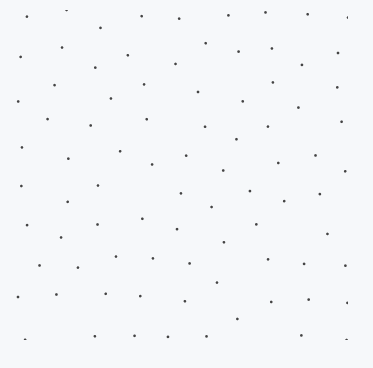
The last thing is to implement a function, which updates all probe particles
advectParticles[v_, pts_, \[Delta]t_ : 0.02] :=
 Map[Function[p, p + \[Delta]t (bilinearInterpolation[v, p])], pts]
Complete Real-Time fluid simulation
Wrapping everything up together with the divergence solver from the previous part, we can finally assemble the model
removeDivergence[grid_] :=
 With[{(*safety checks,which enforce closed boundaries*)
   take = Function[{array, x, y},
     If[x >= 1 && x <= Length[grid] && y >= 1 && y <= Length[grid],
      array[[x, y]], {0, 0}]]},
  MapIndexed[
   Function[{val, i},
    val + ((1)/(8.0)) (((take[grid, i[[1]] - 1, i[[2]] - 1] +
             take[grid, i[[1]] + 1, i[[2]] + 1]) . {1, 1}) {1,
          1} + ((take[grid, i[[1]] - 1, i[[2]] + 1] +
             take[grid, i[[1]] + 1,
              i[[2]] - 1]) . {1, -1}) {1, -1} + (take[grid,
            i[[1]] - 1, i[[2]]] + take[grid, i[[1]] + 1, i[[2]]] -
           take[grid, i[[1]], i[[2]] - 1] -
           take[grid, i[[1]], i[[2]] + 1]) {2, -2} +
        take[grid, i[[1]], i[[2]]]  (-4))], grid, {2}]]
TL;DR Here is the final code
fgrid = Table[{0., 0.}, {i, 15}, {j, 15}];
fngrid =
  fgrid //
   NumericArray; (*introduce a copy of fgrid wrapped as NumericArray*)

(*NumericArray is always faster than a normal List*)

fcolors = Table[1.0, {Length[fgrid]}, {Length[fgrid]}];

start = {1, 1};
drawing = False;
dest = {0, 0};
ffps = 0;

particles =
  RandomPointConfiguration[HardcorePointProcess[10000, 0.4, 2],
    Rectangle[{1 + 4, 1 + 4}, {15 - 4, 15 - 4}],
    Method -> {"LengthOfRun" -> 10000000}]["Points"];

With[{win =
   CurrentWindow[],(*save the current window to append graphics*)
  currentCell = ResultCell[]},
 EventHandler[
  win, {"Closed" ->
    Function[Null,
     Delete[currentCell] (*remove output cell if a notebook has been \
closed*)(*this will prevent the animation running uncontrollably on \
the next start*)]}];
 Graphics[{Arrowheads[Medium/2],
   Table[With[{i = i,
      j = j},(*BB[*)(*now we have dynamic Hue and dynamic Arrow*)
     Offload[{Hue[fcolors[[i]][[j]]],
       Arrow[{{i, j}, {i, j} + fngrid[[i]][[j]]}]}]], {i, 15}, {j,
     15}],(*attach listeners to a user's mouse to manipulate the grid*)
   EventHandler[
    Graphics`Canvas[], {"mouseup" ->
      Function[xy,
       With[{v = -Normalize[start - xy]},
        Do[(*draw a line of velocities*)
          With[{p = Round /@ ((xy - start)  a + start)},
            If[p[[1]] <= 15 && p[[1]] >= 1 && p[[2]] <= 15 &&
               p[[2]] >= 1,
              fgrid[[p[[1]], p[[2]]]] = {v[[1]], v[[2]]};];];, {a, 0,
           1, 0.1}];];
       Delete[drawing];(*delete temporal arrow*)drawing = False;],
     "mousemove" -> Function[xy, dest = xy;],
     "mousedown" -> Function[xy, start = xy;
       dest = xy;
       If[drawing =!= False, Delete[drawing]];
       (*append GUI's arrow to existing canvas*)
       drawing =
        FrontSubmit[{AbsoluteThickness[3], Gray,
          Arrow[{xy, dest // Offload}]}, MetaMarker["fcanvas"],
         "Window" -> win,
         "Tracking" ->
          True (*enable tracking of created object*)];]}],(*sync with \
browser's repaint cycle and update of fps label*)
   AnimationFrameListener[ffps // Offload, "Event" -> "fframe"],
   r["fcanvas"], PointSize[0.02], Point[particles // Offload],
   Text[ffps // Offload, {0, 0}]}, Controls -> False,
  ImageSize -> 500, PlotRange -> {{-0.5, 15.5}, {-0.5, 15.5}},
  ImagePadding -> None,
  TransitionDuration -> 35 (*since the simulation is slow,
  we have to interpolate*)]]

(*subscribe to animation event*)

ftime = AbsoluteTime[];

(*1 advection per 2 removeDivergence*)
fpipeline =
  Composition[removeDivergence, removeDivergence, advect[#, #, 0.2] &];

EventHandler["fframe",
  Function[Null,(*apply the whole pipline as a single function*)
   fgrid = fpipeline[fgrid];
   fngrid = fgrid // NumericArray;(*speed up data-
   transfer by packaging array*)
   fcolors =
    Map[Function[
       val, ((\[Pi] + 2.0  ToPolarCoordinates[val] //
           Last)/(3.0  \[Pi]))], fgrid, {2}] // NumericArray;
   (*2 times advection*)
   particles =
    With[{p = advectParticles[fgrid, particles // Normal, 0.3]},
     advectParticles[fgrid, p, 0.3] // NumericArray];
   ffps = (((ffps + 1/(AbsoluteTime[] - ftime)))/(2.0)) // Round;
   ftime = AbsoluteTime[];]];
Use your mouse to draw velocity vectors like on the video 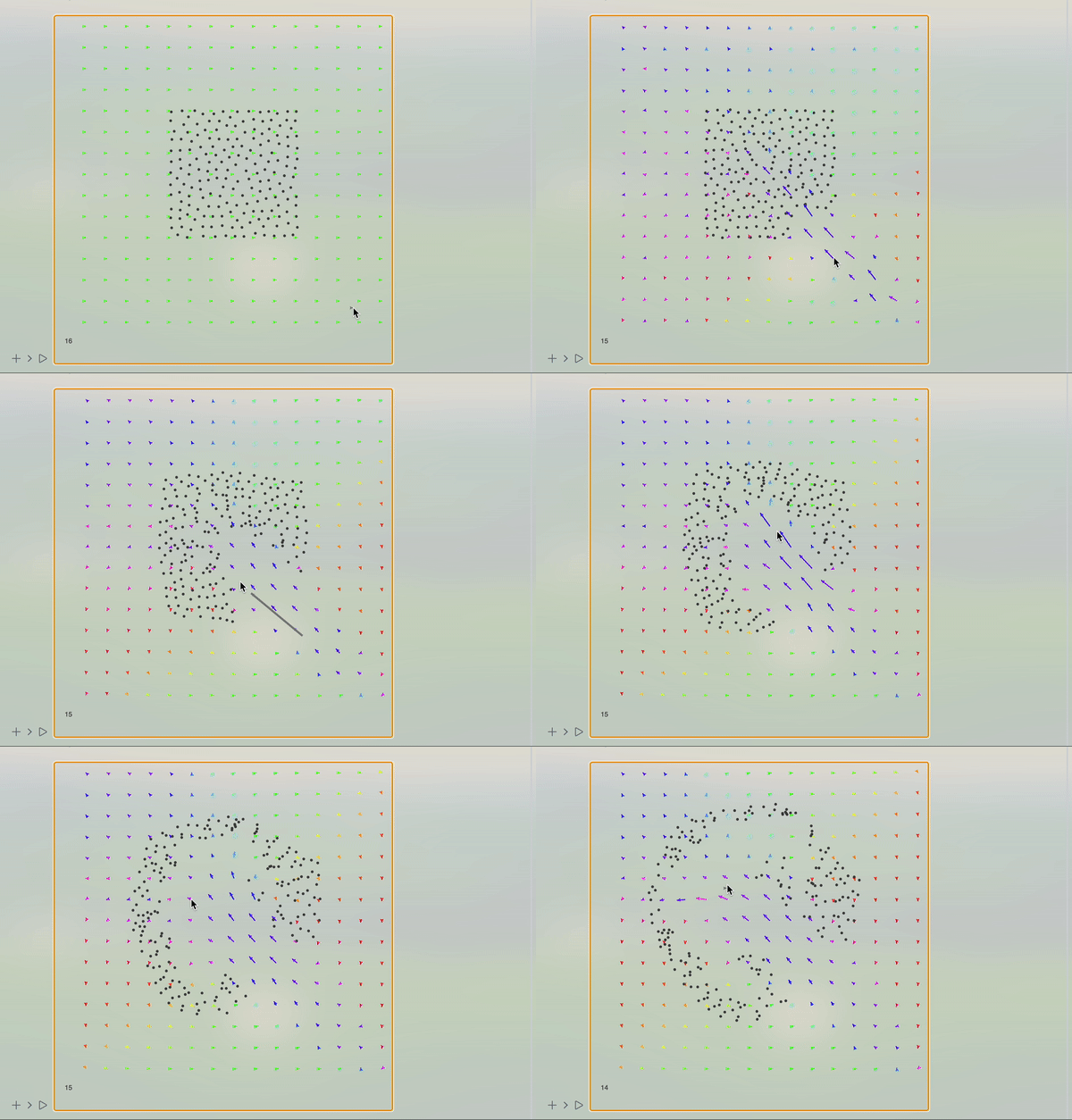
There is still a lot that can be improved further. Especially advection and the code for removing divergence can be optimized and compiled as well.
Optimizations
Since all our main functions used in the animation loop are dealing only with numerics, one can apply Compile to them. With some minor changes made (which unfortunately make the code a bit ugly, because not all functions are compilable) we have
advect =
  Compile[{{v, _Real, 3}, {u, _Real, 3}, {\[Delta]t, _Real, 0}},
   With[{max = Length[v]},
    With[{},
     Table[With[{v1 = ((If[i - 1 >= 1, v[[i - 1, j]], {0., 0.}] +
               v[[i, j]])/(2.0)) . {1, 0},
         v2 = ((If[j + 1 <= max, v[[i, j + 1]], {0., 0.}] +
               v[[i, j]])/(2.0)) . {0, -1},
         v3 = ((If[i + 1 <= max, v[[i + 1, j]], {0., 0.}] +
               v[[i, j]])/(2.0)) . {-1, 0},
         v4 = ((If[j - 1 >= 1, v[[i, j - 1]], {0., 0.}] +
               v[[i, j]])/(2.0)) . {0, 1}, org = u[[i, j]]},
        org + (v1  If[v1 > 0, If[i - 1 >= 1, u[[i - 1, j]], {0., 0.}],
               org] + v3  If[v3 > 0,
              If[i + 1 <= max, u[[i + 1, j]], {0., 0.}], org] +
            v4  If[v4 > 0, If[j - 1 >= 1, u[[i, j - 1]], {0., 0.}],
              org] + v2  If[v2 > 0,
              If[j + 1 <= max, u[[i, j + 1]], {0., 0.}],
              org])  \[Delta]t], {i, max}, {j, max}] // Chop]]];
removeDivergence =
  Compile[{{grid, _Real, 3}},
   With[{max = grid // Length},
    MapIndexed[
     Function[{val, i},
      val + ((1)/(8.0))  (((If[
                i[[1]] - 1 >= 1 && i[[1]] - 1 <= max &&
                 i[[2]] - 1 >= 1 && i[[2]] - 1 <= max,
                grid[[i[[1]] - 1, i[[2]] - 1]], {0., 0.}] +
               If[i[[1]] + 1 >= 1 && i[[1]] + 1 <= max &&
                 i[[2]] + 1 >= 1 && i[[2]] + 1 <= max,
                grid[[i[[1]] + 1, i[[2]] + 1]], {0., 0.}]) . {1,
              1}) {1, 1} + ((If[
                i[[1]] - 1 >= 1 && i[[1]] - 1 <= max &&
                 i[[2]] + 1 >= 1 && i[[2]] + 1 <= max,
                grid[[i[[1]] - 1, i[[2]] + 1]], {0., 0.}] +
               If[i[[1]] + 1 >= 1 && i[[1]] + 1 <= max &&
                 i[[2]] - 1 >= 1 && i[[2]] - 1 <= max,
                grid[[i[[1]] + 1, i[[2]] - 1]], {0.,
                 0.}]) . {1, -1}) {1, -1} + (If[
              i[[1]] - 1 >= 1 && i[[1]] - 1 <= max,
              grid[[i[[1]] - 1, i[[2]]]], {0., 0.}] +
             If[i[[1]] + 1 >= 1 && i[[1]] + 1 <= max,
              grid[[i[[1]] + 1, i[[2]]]], {0., 0.}] -
             If[i[[2]] - 1 >= 1 && i[[2]] - 1 <= max,
              grid[[i[[1]], i[[2]] - 1]], {0., 0.}] -
             If[i[[2]] + 1 >= 1 && i[[2]] + 1 <= max,
              grid[[i[[1]], i[[2]] + 1]], {0., 0.}]) {2, -2} +
          grid[[i[[1]], i[[2]]]]  (-4))], grid, {2}]]];
and
bilinearInterpolation =
  Compile[{{array, _Real, 3}, {v, _Real, 1}},
   Module[{rows, cols, x = v[[2]], y = v[[1]], x1, x2, y1, y2, fQ11,
     fQ12, fQ21,
     fQ22},(*Get the dimensions of the array*){rows,
      cols} = {Length[array], Length[array]};
    (*Clip points to the boundaries*)x = Clip[x, {1, cols}];
    y = Clip[y, {1, rows}];
    (*Find the bounding indices*)x1 = Floor[x];
    x2 = Ceiling[x];
    y1 = Floor[y];
    y2 = Ceiling[y];
    (*Get the values at the four corners*)fQ11 = array[[y1, x1]];
    fQ12 = array[[y2, x1]];
    fQ21 = array[[y1, x2]];
    fQ22 = array[[y2, x2]];
    (*Perform bilinear interpolation*)
    If[x2 == x1,
     If[y2 == y1, fQ11,
      1/(2  (y2 - y1))*(fQ11  (y2 - y) + fQ21  (y2 - y) +
         fQ12  (y - y1) + fQ22  (y - y1))],
     If[y2 == y1,
      1/(2  (x2 - x1))*(fQ11  (x2 - x) + fQ21  (x - x1) +
         fQ12  (x2 - x) + fQ22  (x - x1)),
      1/((x2 - x1)  (y2 - y1))*(fQ11  (x2 - x)  (y2 - y) +
         fQ21  (x - x1)  (y2 - y) + fQ12  (x2 - x)  (y - y1) +
         fQ22  (x - x1)  (y - y1))]]]];
After that the main bottleneck is still the way how we draw and update SVG graphics (as well as WebSocket connection latency). However, these changes improves average FPS from up to on my Mac Air M1.17-2430-35