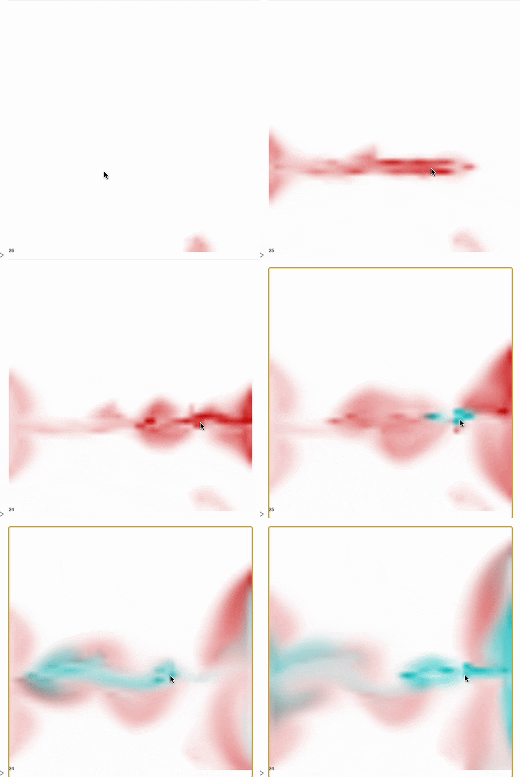
In this post we will apply some optimizations to the code, expand the resolution and switch to immediate mode of graphics rendering.
Measure and optimize
Let us try to estimate the time we need to do our normal calculations on divergence, advection and bilinear interpolation
ClearAll[advect]; ClearAll[removeDivergence]; ClearAll[bilinearInterpolation];

advect[v_, u_, δt_:0.1] := With[{max = Length[v]}, With[{
  take = Function[{array, x,y}, If[x >= 1 && x <= max && y >= 1 && y <= max, array[[x,y]], array[[1,1]] 0.]]
},
  Table[

    With[{
      v1 = ((take[v, i-1, j] + take[v, i, j])/(2.0)).{1,0},
      v2 =  ((take[v, i, j+1] + take[v, i, j])/(2.0)).{0,-1},
      v3 =  ((take[v, i+1, j] + take[v, i, j])/(2.0)).{-1,0},
      v4 =  ((take[v, i, j-1] + take[v, i, j])/(2.0)).{0,1},
      org = u[[i,j]]
    },

      org + (

        v1 Piecewise[{{take[u, i-1, j],v1 > 0},{org,True}}] + v3 Piecewise[{{take[u, i+1, j],v3 > 0},{org,True}}]  +

        v4 Piecewise[{{take[u, i, j-1],v4 > 0},{org,True}}] + v2 Piecewise[{{take[u, i, j+1],v2 > 0},{org,True}}]

      ) δt
    ]

  , {i, max}, {j, max}] // Chop
 ]]

 removeDivergence[grid_] := With[{
  (*safety checks, which enforce closed boundaries*)
  take = Function[{array, x,y}, If[x >= 1 && x <= Length[grid] && y >= 1 && y <= Length[grid], array[[x,y]], {0,0}]]
},
  MapIndexed[Function[{val, i},
    val + ((1)/(8.0)) (
      ((take[grid, i[[1]] - 1, i[[2]] - 1] + take[grid, i[[1]] + 1, i[[2]] + 1]).{1,1}){1,1} +

      ((take[grid, i[[1]] - 1, i[[2]] + 1] + take[grid, i[[1]] + 1, i[[2]] - 1]).{1,-1}){1,-1} +

      (take[grid, i[[1]]-1, i[[2]]] + take[grid, i[[1]]+1, i[[2]]] - take[grid, i[[1]], i[[2]]-1] - take[grid, i[[1]], i[[2]]+1]){2,-2} + take[grid, i[[1]], i[[2]]] (-4)

    )
  ], grid, {2}]
]

bilinearInterpolation[array_, {x0_, y0_}] := Module[
  {rows, cols, x = y0, y = x0, x1, x2, y1, y2, fQ11, fQ12, fQ21, fQ22},

  (* Get the dimensions of the array *)
  {rows, cols} = Take[Dimensions[array], 2];

  (* Clip points to the boundaries *)
  x = Clip[x, {1, cols}];
  y = Clip[y, {1, rows}];

  (* Find the bounding indices *)
  x1 = Floor[x];
  x2 = Ceiling[x];
  y1 = Floor[y];
  y2 = Ceiling[y];

  (* Get the values at the four corners *)
  fQ11 = array[[y1, x1]];
  fQ12 = array[[y2, x1]];
  fQ21 = array[[y1, x2]];
  fQ22 = array[[y2, x2]];

  (* Perform bilinear interpolation *)
  If[x2 == x1,
    If[y2 == y1,
      fQ11,
      1/(2 (y2 - y1)) * (
        fQ11 (y2 - y) +
        fQ21 (y2 - y) +
        fQ12 (y - y1) +
        fQ22 (y - y1)
      )
    ],
    If[y2 == y1,
      1/(2 (x2 - x1)) * (
        fQ11 (x2 - x) +
        fQ21 (x - x1) +
        fQ12 (x2 - x) +
        fQ22 (x - x1)
      ),
      1/((x2 - x1) (y2 - y1)) * (
        fQ11 (x2 - x) (y2 - y) +
        fQ21 (x - x1) (y2 - y) +
        fQ12 (x2 - x) (y - y1) +
        fQ22 (x - x1) (y - y1)
      )
    ]
  ]
]

advectParticles[v_, pts_, δt_:0.02] := Map[Function[p, p + δt (bilinearInterpolation[v, p])], pts]
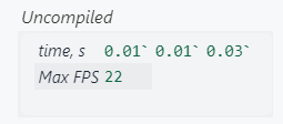
For a single run we have
runTest[title_] := With[{},
  testGrid = Table[{0.,0.}, {i,15}, {j,15}];
  testParticles = Table[RandomReal[{1,15}, 2], {i,1000}];

  timing = {0., 0., 0.};

  timing[[1]] = -AbsoluteTime[];
  testGrid = advect[testGrid, testGrid, 0.2];
  timing[[1]] += AbsoluteTime[];

  timing[[2]] = -AbsoluteTime[];
  testGrid = removeDivergence[testGrid];
  timing[[2]] += AbsoluteTime[];

  timing[[3]] = -AbsoluteTime[];
  testParticles = advectParticles[testGrid, testParticles, 0.2];
  timing[[3]] += AbsoluteTime[];

  {
    Style[title, Italic, 12],

    Flatten /@ {
      {Style["time, s", Italic], Round[timing, 0.001]},
      {Style["Max FPS", Italic], Round[1 / (timing // Total), 1]}
    } // TableView
  } // Column
];

runTest["Uncompiled"]
Compile
Most probably for pure function JIT compiler should kick in, however, not all expressions are compilable in our case. We can make them by removing function declaration within the Module and replacing Piecewise with just a normal If statement.
It makes our code looks less readable, but the result worth it
advect = Compile[{{v, _Real, 3}, {u, _Real, 3}, {δt, _Real, 0}} , With[{max = Length[v]}, With[{

},
  Table[

    With[{
      (* here we add a lot of manual check for boundary condition *)
      v1 = ( ((If[i-1 >= 1, v[[i-1, j]], {0.,0.}] + v[[i, j]])/(2.0))).{1,0},
      v2 =  ((If[j+1 <= max, v[[i, j+1]], {0.,0.}] + v[[i, j]])/(2.0)).{0,-1},
      v3 =  ((If[i+1 <= max, v[[i+1, j]], {0.,0.}] + v[[i, j]])/(2.0)).{-1,0},
      v4 =  ((If[j-1 >= 1, v[[i, j-1]], {0.,0.}] + v[[i, j]])/(2.0)).{0,1},
      org = u[[i,j]]
    },

      org +  (
        (* here we add a lot of manual check for boundary condition *)

        v1 (If[v1 >0, If[i-1 >= 1, u[[i-1, j]], {0.,0.} ], org])

        + v3 (If[v3>0,If[i+1 <= max, u[[i+1, j]], {0.,0.} ], org])+

        v4 If[v4 >0, If[j-1 >= 1, u[[i, j-1]], {0.,0.} ], org]

        + v2 If[v2>0, If[j+1 <= max, u[[i, j+1]], {0.,0.} ], org]

      ) δt
    ]

  , {i, max}, {j, max}] // Chop
 ]]];

removeDivergence = Compile[{{grid, _Real, 3}}, With[{
  max = grid // Length
},
  MapIndexed[Function[{val, i},
    val + ((1)/(8.0)) (
      (
        (
          (* here we add a lot of manual check for boundary condition *)(*,*)
          If[i[[1]] - 1 >= 1 && i[[1]] - 1 <= max && i[[2]] - 1 >= 1 && i[[2]] - 1 <= max, grid[[i[[1]] - 1, i[[2]] - 1]], {0.,0.}]

          + If[i[[1]] + 1 >=1 && i[[1]] + 1 <= max && i[[2]] + 1 >= 1 && i[[2]] + 1 <= max, grid[[i[[1]] + 1, i[[2]] + 1]], {0.,0.}]

        ).{1,1}

      ){1,1} +

      (
        (
          (* here we add a lot of manual check for boundary condition *)
          If[i[[1]] - 1 >= 1 && i[[1]] - 1 <= max && i[[2]] + 1 >= 1 && i[[2]] + 1 <= max, grid[[i[[1]] - 1, i[[2]] + 1]], {0.,0.}]

          + If[i[[1]] + 1 >= 1 && i[[1]] + 1 <= max && i[[2]] - 1 >= 1 && i[[2]] - 1 <= max, grid[[i[[1]] + 1, i[[2]] - 1]], {0.,0.}]

        ).{1,-1}

      ){1,-1} +

      (
        (If[i[[1]]-1 >= 1 && i[[1]]-1 <= max, grid[[i[[1]]-1, i[[2]] ]], {0.,0.}])

        + If[i[[1]]+1 >= 1 && i[[1]]+1 <= max, grid[[ i[[1]]+1, i[[2]] ]], {0.,0.}]

        - If[i[[2]]-1 >= 1 && i[[2]]-1 <= max, grid[[ i[[1]], i[[2]]-1 ]], {0.,0.}]

        - If[i[[2]]+1 >= 1 && i[[2]]+1 <= max, grid[[i[[1]], i[[2]]+1]], {0.,0.}]

      ){2,-2}

        + grid[[ i[[1]], i[[2]] ]] (-4)

    )
  ], grid, {2}]
]];

bilinearInterpolation = Compile[{{array, _Real, 3}, {v, _Real, 1}},
(* no big changes here *)
Module[
  {rows, cols, x = v[[2]], y = v[[1]], x1, x2, y1, y2, fQ11, fQ12, fQ21, fQ22},

  (* Get the dimensions of the array *)
  {rows, cols} = {Length[array], Length[array]};

  (* Clip points to the boundaries *)
  x = Clip[x, {1, cols}];
  y = Clip[y, {1, rows}];

  (* Find the bounding indices *)
  x1 = Floor[x];
  x2 = Ceiling[x];
  y1 = Floor[y];
  y2 = Ceiling[y];

  (* Get the values at the four corners *)
  fQ11 = array[[y1, x1]];
  fQ12 = array[[y2, x1]];
  fQ21 = array[[y1, x2]];
  fQ22 = array[[y2, x2]];

  (* Perform bilinear interpolation *)
  If[x2 == x1,
    If[y2 == y1,
      fQ11,
      1/(2 (y2 - y1)) * (
        fQ11 (y2 - y) +
        fQ21 (y2 - y) +
        fQ12 (y - y1) +
        fQ22 (y - y1)
      )
    ],
    If[y2 == y1,
      1/(2 (x2 - x1)) * (
        fQ11 (x2 - x) +
        fQ21 (x - x1) +
        fQ12 (x2 - x) +
        fQ22 (x - x1)
      ),
      1/((x2 - x1) (y2 - y1)) * (
        fQ11 (x2 - x) (y2 - y) +
        fQ21 (x - x1) (y2 - y) +
        fQ12 (x2 - x) (y - y1) +
        fQ22 (x - x1) (y - y1)
      )
    ]
  ]
]];
Let us test it again!
runTest["Compiled"]
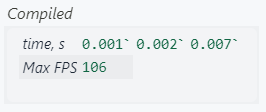
x5 time faster
However, one should note, that this is still not a machine code, but rather byte-code of Wolfram Kernel internal command representation or something similar to that.
One can go futher and force WL to compile it to C and then link automatically. This will probably require to have gcc or clang installed on your system
advect = Compile[{{v, _Real, 3}, {u, _Real, 3}, {δt, _Real, 0}} , With[{max = Length[v]}, With[{

},
  Table[

    With[{
      v1 =  ((If[i-1 >= 1, v[[i-1, j]], {0.,0.}] + v[[i, j]])/(2.0)).{1,0},
      v2 =  ((If[j+1 <= max, v[[i, j+1]], {0.,0.}] + v[[i, j]])/(2.0)).{0,-1},
      v3 =  ((If[i+1 <= max, v[[i+1, j]], {0.,0.}] + v[[i, j]])/(2.0)).{-1,0},
      v4 =  ((If[j-1 >= 1, v[[i, j-1]], {0.,0.}] + v[[i, j]])/(2.0)).{0,1},
      org = u[[i,j]]
    },

      org +  (

        v1 If[v1 >0, If[i-1 >= 1, u[[i-1, j]], {0.,0.} ], org]  + v3 If[v3>0,If[i+1 <= max, u[[i+1, j]], {0.,0.} ], org]+

        v4 If[v4 >0, If[j-1 >= 1, u[[i, j-1]], {0.,0.} ], org] + v2 If[v2>0, If[j+1 <= max, u[[i, j+1]], {0.,0.} ], org]

      ) δt
    ]

  , {i, max}, {j, max}] // Chop
 ]] , CompilationOptions -> {"InlineExternalDefinitions" -> True},
    "CompilationTarget" -> "C", "RuntimeOptions" -> "Speed"];

removeDivergence = Compile[{{grid, _Real, 3}}, With[{
  max = grid // Length
},
  MapIndexed[Function[{val, i},
    val + ((1)/(8.0)) (
      (
        (
          If[i[[1]] - 1 >= 1 && i[[1]] - 1 <= max && i[[2]] - 1 >= 1 && i[[2]] - 1 <= max, grid[[i[[1]] - 1, i[[2]] - 1]], {0.,0.}]

          + If[i[[1]] + 1 >=1 && i[[1]] + 1 <= max && i[[2]] + 1 >= 1 && i[[2]] + 1 <= max, grid[[i[[1]] + 1, i[[2]] + 1]], {0.,0.}]

        ).{1,1}

      ){1,1} +

      (
        (
          If[i[[1]] - 1 >= 1 && i[[1]] - 1 <= max && i[[2]] + 1 >= 1 && i[[2]] + 1 <= max, grid[[i[[1]] - 1, i[[2]] + 1]], {0.,0.}]

          + If[i[[1]] + 1 >= 1 && i[[1]] + 1 <= max && i[[2]] - 1 >= 1 && i[[2]] - 1 <= max, grid[[i[[1]] + 1, i[[2]] - 1]], {0.,0.}]

        ).{1,-1}

      ){1,-1} +

      (
        If[i[[1]]-1 >= 1 && i[[1]]-1 <= max, grid[[i[[1]]-1, i[[2]] ]], {0.,0.}]

        + If[i[[1]]+1 >= 1 && i[[1]]+1 <= max, grid[[ i[[1]]+1, i[[2]] ]], {0.,0.}]

        - If[i[[2]]-1 >= 1 && i[[2]]-1 <= max, grid[[ i[[1]], i[[2]]-1 ]], {0.,0.}]

        - If[i[[2]]+1 >= 1 && i[[2]]+1 <= max, grid[[i[[1]], i[[2]]+1]], {0.,0.}]

      ){2,-2}

        + grid[[ i[[1]], i[[2]] ]] (-4)

    )
  ], grid, {2}]
], CompilationOptions -> {"InlineExternalDefinitions" -> True},
    "CompilationTarget" -> "C",   "RuntimeOptions" -> "Speed"];


bilinearInterpolation = Compile[{{array, _Real, 3}, {v, _Real, 1}}, Module[
  {rows, cols, x = v[[2]], y = v[[1]], x1, x2, y1, y2, fQ11, fQ12, fQ21, fQ22},

  (* Get the dimensions of the array *)
  {rows, cols} = {Length[array], Length[array]};

  (* Clip points to the boundaries *)
  x = Clip[x, {1, cols}];
  y = Clip[y, {1, rows}];

  (* Find the bounding indices *)
  x1 = Floor[x];
  x2 = Ceiling[x];
  y1 = Floor[y];
  y2 = Ceiling[y];

  (* Get the values at the four corners *)
  fQ11 = array[[y1, x1]];
  fQ12 = array[[y2, x1]];
  fQ21 = array[[y1, x2]];
  fQ22 = array[[y2, x2]];

  (* Perform bilinear interpolation *)
  If[x2 == x1,
    If[y2 == y1,
      fQ11,
      1/(2 (y2 - y1)) * (
        fQ11 (y2 - y) +
        fQ21 (y2 - y) +
        fQ12 (y - y1) +
        fQ22 (y - y1)
      )
    ],
    If[y2 == y1,
      1/(2 (x2 - x1)) * (
        fQ11 (x2 - x) +
        fQ21 (x - x1) +
        fQ12 (x2 - x) +
        fQ22 (x - x1)
      ),
      1/((x2 - x1) (y2 - y1)) * (
        fQ11 (x2 - x) (y2 - y) +
        fQ21 (x - x1) (y2 - y) +
        fQ12 (x2 - x) (y - y1) +
        fQ22 (x - x1) (y - y1)
      )
    ]
  ]
] , CompilationOptions -> {"InlineExternalDefinitions" -> True},
    "CompilationTarget" -> "C","RuntimeOptions" -> "Speed"];
Now we have new results
runTest["Compiled + C"]
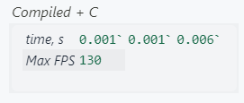
x6 time faster
We gained a bit of speed; we will see more difference once the grid is expanded and more iterations are needed.
Immediate Graphics Mode
This only means, that we will do all rendering of our primitives by ourself. The graphics API will only display the rendered frame we crafted on Wolfram Kernel. The last also meant we migh have to transfer much more data over WebSockets to frontend.
Let me show you a simple example
Table[Clip[(Power[x,2] + Power[y,2]) - Power[10,2], {0, 1}], {x,-10,10, 0.5}, {y,-10,10, 0.5}];
Image[%, Magnification -> 5, Antialiasing->False]
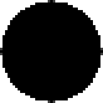
Here we used so-called SDF method for drawing graphics. We iterate over all posiitons of pixels in reactangle, produce brightness values and then send them to Image, which copies them into a texture on GPU.
We can use all 4 (RGBA) color channels to draw our picture
Table[{
  Clip[(Power[x,2] + Power[y,2]) - Power[10,2], {0, 1}],
  Clip[(Power[x,2] + Power[y,2]) - Power[5,2], {0, 1}],
  Clip[(Power[x,2] + Power[y,2]) - Power[3,2], {0, 1}],
  Clip[(Power[x,2] + Power[y,2]) - Power[1,2], {0, 1}]
}, {x,-10,10, 0.5}, {y,-10,10, 0.5}];
Image[%, Magnification -> 5, Antialiasing->False]

For the best performance use NumericArray, since it packs all numberic data to a more compact form
Table[{
  Clip[(Power[x,2] + Power[y,2]) - Power[10,2], {0, 1}],
  Clip[(Power[x,2] + Power[y,2]) - Power[5,2], {0, 1}],
  Clip[(Power[x,2] + Power[y,2]) - Power[3,2], {0, 1}],
  Clip[(Power[x,2] + Power[y,2]) - Power[1,2], {0, 1}]
}, {x,-10,10, 0.5}, {y,-10,10, 0.5}];
Image[NumericArray[%, "Real32"], Magnification -> 5, Antialiasing->False]
Dynamic image
There is a usual way on how to update our Image - using Offload technique as we did before
Tip: Real values takes more time to deserialize on frontend, we will use UnsignedInteger8
serialize[arr_List] := NumericArray[arr, "UnsignedInteger8", "ClipAndRound"];

buffer = Table[255.0 {
  Clip[(Power[x,2] + Power[y,2]) - Power[10,2], {0, 1}],
  Clip[(Power[x,2] + Power[y,2]) - Power[5,2], {0, 1}],
  Clip[(Power[x,2] + Power[y,2]) - Power[3,2], {0, 1}],
  Clip[(Power[x,2] + Power[y,2]) - Power[1,2], {0, 1}]
}, {x,-10,10, 0.5}, {y,-10,10, 0.5}] // serialize;

Image[buffer // Offload, "Byte", Magnification -> 5, Antialiasing->False]
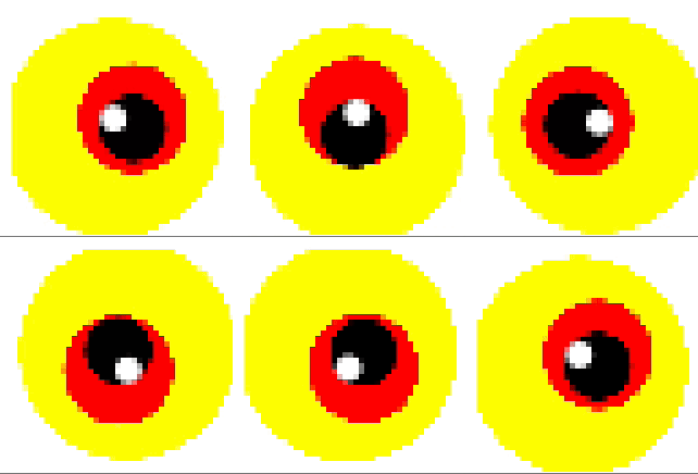
Now we can easily update our image by setting new values to buffer
t := AbsoluteTime[];

task = SetInterval[
  buffer = Table[255.0 {
    Clip[(Power[(x + Cos[t]),2] + Power[(y - Sin[t]),2]) - Power[3,2], {0, 1}],
    Clip[(Power[(x - Cos[t]),2] + Power[(y - Sin[t]),2]) - Power[5,2], {0, 1}],
    Clip[(Power[(x + Cos[t]),2] + Power[(y + Sin[t]),2]) - Power[10,2], {0, 1}],
    Clip[(Power[(x - Cos[t]),2] + Power[(y + Sin[t]),2]) - Power[1,2], {0, 1}]
  }, {x,-10,10, 0.5}, {y,-10,10, 0.5}] // serialize;
, 100];

SetTimeout[TaskRemove[task], 10000];
If you made that far, congratulations. Now you have learned how to do the software rendering.
Please, never do software rendering. It is slow and basically is a waste of resources of your CPU, which was not designed for rendering graphics. Use it only for educational purposes, small images or complex calulations, which are not possible to do using GPU.
Virtual Ink
To visualize velocity field, one can actually use another scalar field instead of 1000 probing balls. This scalar field is easy to imagine: ink or dye or goo, which fell into a water and now is carried by the steams of fluid

We already know how to solve advection equation. Our function advect is used for modelling the momentum of fluid, which is a 2D vector field... Why not then to use two kinds of ink?
ink = Table[{0.,0.}, {i,50}, {j,50}];

(* transform to "byte" format *)
nink = NumericArray[Map[255.0 {#[[1]], 0., #[[2]]} &, ink, {2}], "UnsignedInteger8", "ClipAndRound"];
Then we can directly visualize nink scalar field instead of drawing many many arrows and dots. In this way we will utilize fully our expensive software rendering.
TL;DR Final program
vgrid = Table[{0.,0.}, {i,50}, {j,50}];

ink = 0. ink;
nink = NumericArray[Map[255.0 {#[[1]], 0., #[[2]]} &, ink, {2}], "UnsignedInteger8", "ClipAndRound"];

dest = {0,0};
cink = {1.0,0.2};
vfps = 0;

With[{
  win = CurrentWindow[],
  currentCell = ResultCell[]
},

  EventHandler[win, {"Closed" -> Function[Null,
    Delete[currentCell] (* remove output cell if a notebook has been closed *)
    (* this will prevent the animation running uncontrollably on the next start *)
  ]}];

  Graphics[{

    (*attach listeners to a user's mouse to manipulate the grid*)
    EventHandler[Graphics`Canvas[], {
      "click" -> Function[Null,
        cink = cink // Reverse;
      ],

      "mousemove" -> Function[pos, With[{
          xy = {50.0 - pos[[2]], pos[[1]]}
        },
          With[{p = Round[xy]},
            If[p[[1]] <= 50-1 && p[[1]] >=2 && p[[2]] <=50-1 && p[[2]] >=2,
                (* accelerate the fluid *)
                vgrid[[p[[1]],p[[2]]]] = Normalize[(xy - dest)];

                (* add some ink *)
                ink[[p[[1]],p[[2]]]] = cink;
                ink[[p[[1]]+1,p[[2]]]] = cink;
                ink[[p[[1]]-1,p[[2]]]] = cink;
                ink[[p[[1]],p[[2]]+1]] = cink;
                ink[[p[[1]],p[[2]]+1]] = cink;
            ];

          ];

          dest = xy;
        ] ]
    }],

    (*sync with browser's repaint cycle and update of fps label*)
    AnimationFrameListener[vfps // Offload, "Event"->"vframe"],

    (*insert our Image*)
    Inset[

      Image[nink // Offload, "Byte", Magnification->10]

    , {0,0}, {0,0}, {500,500},

      (* do not apply any transformation. keep the original size *)
      ViewMatrix->None
    ],

    Text[vfps // Offload, {0,0}]


  },
    Controls->False,
    ImageSize->500,
    PlotRange->{{0,50}, {0,50}},
    ImagePadding->None
  ]
]

(* subscribe to animation event *)

vtime = AbsoluteTime[];

EventHandler["vframe", Function[Null,

  vgrid = advect[vgrid,vgrid, 1.0];
  vgrid = removeDivergence[vgrid];
  vgrid = removeDivergence[vgrid];

  ink = With[{a = advect[vgrid, ink, 1.0]}, advect[vgrid, a, 1.0]];
  nink = NumericArray[Map[255.0 {1.0 - #[[2]], 1.0- #[[1]], 1.0 - #[[1]], 1.0} &, ink, {2}], "UnsignedInteger8", "ClipAndRound"];

  vfps = (*FB[*)(((vfps + 1 / (AbsoluteTime[] - vtime)))(*,*)/(*,*)(2.0))(*]FB*) // Round;
  vtime = AbsoluteTime[];
]];
We do here pretty much the same as before; however, there are no longer arrows but a single Inset with a raster dynamic image inside. This places the Image on top of our Graphics canvas. This overlay is helpful since we can still listen to mouse positions and display FPS at a low cost. The fluid goes in the same direction as the mouse
https://jerryi.github.io/wljs-docs/assets/medias/fluid_raster-e1fa9e5abb674313def47863e086ac1f.mov
I (Me - @JerryI) personally believe that we pushed the implementation to the limits of this toy model running on a CPU with an interpretive programming language. The next step definitely should be to utilize GPU compute shaders such as WebGPU, OpenCL, CUDA to calculate bigger fields and pipe the data directly to the canvas. However, this will be another story.