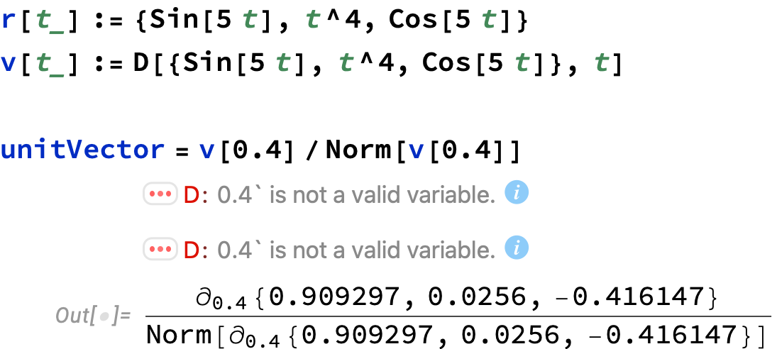
I'll describe how I try to figure out an error like "0.4 is not a valid variable", along the teach-a-person-to-fish school of thought. A possible fix is at the end.
1. The error message
The first thing to understand is the error message. It's often enough to locate the problem. In the older versions, all you got was "D::ivar : 0.4` is not a valid variable. >>", where the ">>" was a link to the documentation page for the error, if it existed. Now you get a helpful three-dot button and the link is now a baby-blue-background "i".

We'll get to the three dots, but first, we have two errors about 0.4 and there exactly two places in the code where 0.4 occurs. 99% sure that the error is located in v[t]. I'd try it: execute v[0.4] by itself. You'll get the same error.
If that isn't enough to figure out what's wrong, the next step is to investigate v[t]. Or if you didn't think of checking v[t], click the three-dot button on the first error (always check the first error first; subsequent errors might be because of the first error). You'll get a popup menu: select "Show Stack Trace." You'll see a sequence of commands that leads to the error. You cannot count on it being self-explanatory, in my experience. But it gives helpful clues. For instance on sees the D[] command that gave the error:

The is the typeset form of the input code D[{0.909297, 0.0256, -0.416147}, 0.4]. One can see something has gone wrong in v[0.4], since there are no formulas or variables to differentiate.
Now it's true, one might get stuck, until one has an idea. I would take apart the code for v[t]. For instance, plug 0.4 in for t in the vector to be differentiated:
{Sin[5 0.4], 0.4^4, Cos[5 0.4]}  (* <-- Note spaces before 0.4; or use * for mult. *)
(* Out[]= {0.909297, 0.0256, -0.416147}  *)
We start to get the idea that t is being plugged in before the derivative is taken. Which is bad.
Tracing the evaluation of v[0.4]
TracePrint[] and Trace[] can trace the evaluation steps of a computation. TracePrint[] is bit more complete. It can also print out a lot, which makes it hard to parse the steps. Trace[], on the other hand, gives the levels of the steps in nested lists, which also can be hard to parse. For a computation with many steps, the outputs of both are difficult to read. They are best used on snippets, when you really want to understand what is happening in a comparatively simple code. By restricting the depth (or "level") to which you trace the execution, you can make the output more readable. I like TracePrint[] in simple cases, because it prints one step per line.
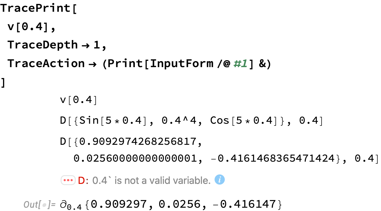
If we trace just the top level, we can see the sequence of transformations of v[0.4], first to plugging in t = 0.4 and then to the erroneous call to D[]:
TracePrint[
 v[0.4],
 TraceDepth -> 1,
 TraceAction -> (Print[InputForm /@ #1] &)
 ]

The option TraceAction -> (Print[InputForm /@ #1] &) is not really necessary. The use of InputForm presents the D[] operator in terms of D[] instead the curly
$\partial_{0.4}$ we see in the Out[]= line. I thought the actual code would be more helpful than the pretty-print version.
Tracing the bad command
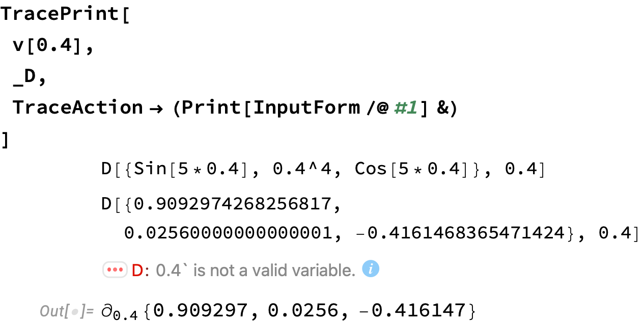
The tracing commands take an optional argument that is a pattern. The output consists of the steps that match the pattern. The pattern _D matches any expression with head D — that is, all expressions of the form D[...]. You don't see all the buildup to the call to D[], but the output is focussed more on the troublesome calls.
TracePrint[
 v[0.4],
 _D,
 TraceAction -> (Print[InputForm /@ #1] &)
 ]

Tracing deeper
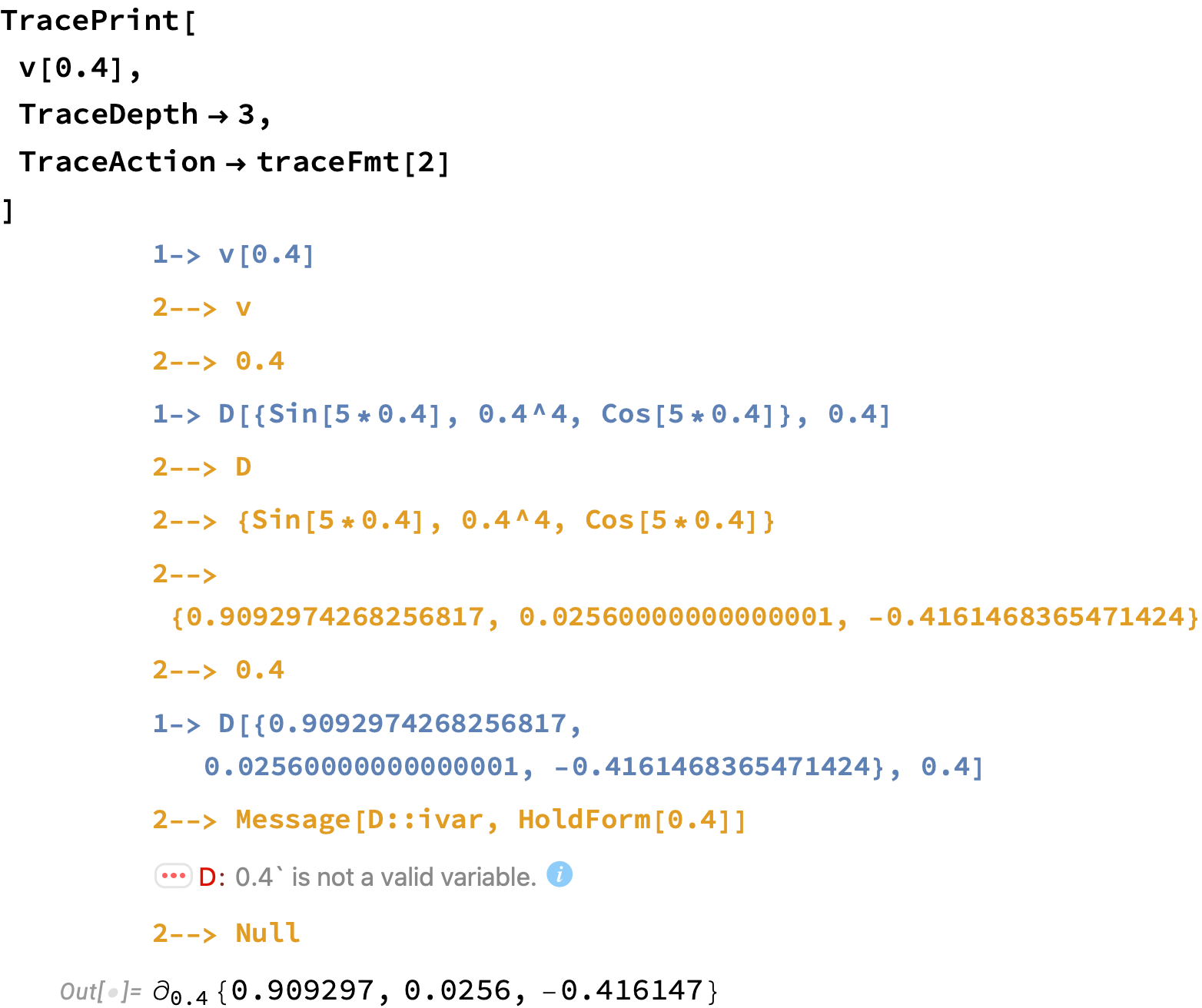
Should you get overexcited about tracing the steps of evaluation, it helps to format the output of TracePrint[]. There is a function TraceLevel[] that gives the current depth of the trace when a step is being printed out by TraceAction. There's a funny thing I don't understand. It turns out with TraceDepth set to some level, you do not always see all the steps at that level; you have to trace at least one level deeper. In this case, to see all the steps at level 2, we need TraceDepth -> 3. Here's a way to highlight the steps as the level goes down and up:
traceFmt // ClearAll;
traceFmt[level_ : Infinity] := (* formats TracePrint output down to level *)
  If[TraceLevel[] <= 1 + level,
   Print[Row[{
       TraceLevel[] - 1,
       StringJoin[Table["-", TraceLevel[] - 1]],
       "> ",
       InputForm /@ #1
       },
      BaseStyle -> {ColorData[97][TraceLevel[] - 1],
        FontWeight -> "SemiBold"}]
     ]
    ] &;

TracePrint[
 v[0.4],
 TraceDepth -> 3,           (* traces down to level 3 *)
 TraceAction -> traceFmt[2] (* prints down to level 2 *)
 ]

Workarounds
Gianluca's suggestion is essentially something like this:
ClearAll[r, v];
r[t_] := {Sin[5 t], t^4, Cos[5 t]};
Block[{t},
 v[t_] = D[{Sin[5 t], t^4, Cos[5 t]}, t]
 ];
I added ClearAll because it's good practice when defining a function to remove all previous definitions and attributes. The use of Block[{t},...] temporarily clears any value that might have been given to t while v[t] is being defined.
A more succinct way:
ClearAll[r, v];
r[t_] := {Sin[5 t], t^4, Cos[5 t]};
Block[{t},
 v[t_] = r'[t];
 ]
An even more succinct way:
And it avoids any trouble with t.
ClearAll[r]; (* Don't really need to clear v in this case *)
r[t_] := {Sin[5 t], t^4, Cos[5 t]};
v = r';

unitVector = Normalize[v[0.4]] (* computes v[0.4] only once *)
Further reading