... But I am getting same contour plot for every time step.
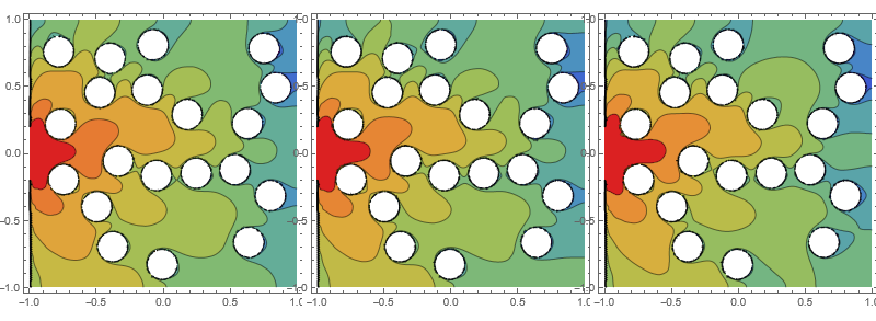
Not quite the same, but similar. If a logarithmic scaling is used, the differences become more visible:
prnt = ContourPlot[cfun[#, x, y], {x, -1, 1}, {y, -1, 1},
     ColorFunction -> "Rainbow", Contours -> 10,
     RegionFunction -> (RegionMember[\[CapitalOmega], {#1, #2}] &),
     PlotRange -> Automatic,
     ScalingFunctions -> "Log"] & /@ {.1, .2, .3};
GraphicsRow[prnt, Spacings -> -15, ImageSize -> 800]