Here is a way to gather timing data from Manipulate[]. The line times[h] = {times[h], SessionTime[]} constructs a linked list (see below), which Mathematica does efficiently. The timings are a bit different than those in my first post, but they should reflect the actual performance of Manipulate[]. I would have expected both to be slower, but GraphicsGrid[] is a bit faster than in the MakeBoxes[] test, although it's still quite a bit slower than Grid[] in both cases.
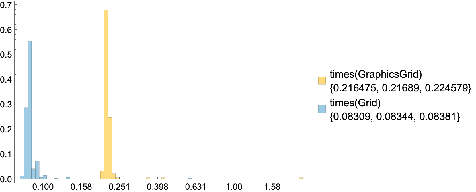
Generate the timing data by continuously varying the slider. There will be extra-long intervals if you stop between sliding. In particular, the time at the beginning is recorded, and then there is a gap between then and when you start sliding. Hence I used Quartiles[] and Histogram[] to estimate the typical behavior. If you collect enough data from sliding the slider, a few extreme values do not affect the Quartiles[].
The Log10[] bin scaling in Histogram[] just made it look prettier, imo. There is no theoretical reason for doing this. And as we're just looking at the difference, there is no theoretical reason not to do it.
Important: Omit times from the TrackedSymbols options or you will get
an infinite Dynamic[]-update loop.
Manipulate[
 times[h] = {times[h], SessionTime[]};
 h[Table[Plot[Sin[2 Pi f t - 2 Pi 0], {t, 0, 6}], 3, 4]],
 {f, 0.5, 2.5},
 {h, {GraphicsGrid, Grid}},
 Initialization :> (Clear[times];
   times[GraphicsGrid] = times[Grid] = Sequence[]),
 TrackedSymbols :> {f, h}
 ]
After manipulating the slider for both heads h, we can visualize the results as follows:
Differences /@ Flatten /@ Values@DownValues@times //
 Histogram[Log10@#, (*scale times before binning*)
   {0.02}, "Probability",
   ChartLegends ->
    Column /@
     Transpose@{HoldForm @@@ Keys@DownValues@times, Quartiles /@ #},
   Ticks -> { (*adjust bin ticks to Log10 scaling*)
     Range[-12, 2, 2]/10. // {#, SetPrecision[10^#, 3]} & // Transpose,
     Automatic}] &
Linked lists
I learned about linked lists a long time ago, but I learned about their form and utility in Mathematica from Leonid Shifrin in this SE post.
Pick a head LL for the linked list. If each datum to be collected is not a List[], then I often use List, which is what I used above. Otherwise, pick a name that will help you remember what you're doing. Then here are the initial step and the update step, with the head testLL:
myLL = testLL[];  (* initialize *)
myLL = testLL[myLL, datum]; (* update *)
Variations:
myLL = Sequence[];  (* no empty container testLL[] *)
myLL = testLL[datum, myLL]; (* reverse order *)
To process the collected data, use Flatten[]:
myData = Flatten[myLL];  (* form: testLL[d1, d2,...] *)
myData = List @@ Flatten[myLL]; (* form: {d1, d2,...} *)
If the data all have the same expression structure, as in the Manipulate[] above, then we can get the first
$n$ data points from the flattened data or as follows (
$n=5$ shown):
Level[times[GraphicsGrid], {-5 - Depth[Last@times[GraphicsGrid]]}] (* raw data *)
Flatten[%] (* flattened data *)
Differences[%] (* delays between updates *)
(*
{{{{{{8749.164792}, 8749.445844}, 8752.260474}, 8752.532522}, 8752.768960}}
{8749.164792, 8749.445844, 8752.260474, 8752.532522, 8752.768960}
{0.281052, 2.814630, 0.272048, 0.236438}
*)

Level[times[Grid], {-5 - Depth[Last@times[Grid]]}] (* raw data *)
Flatten[%] (* flattened data *)
Differences[%] (* delays between updates *)
(*
{{{{{{8778.769036}, 8780.560328}, 8780.679477}, 8780.766351}, 8780.849356}}
{8778.769036, 8780.560328, 8780.679477, 8780.766351, 8780.849356}
{1.791292, 0.119149, 0.086874, 0.083005}
*)
The Histogram[] code leverages the down values of times as a sort of association. The structure looks like the following:
DownValues@times
(*
{HoldPattern[times[GraphicsGrid]] :> {{ ...}, 8777.132784},
 HoldPattern[times[Grid]] :> {{ ...}, 8796.294934}}
*)
I replaced HoldPattern by HoldForm in the keys used in the chart legend.


