Introduction

Your playing a simple game. Make even money bets (a bet that yields an equal positive return for a win or an equal negative return for a loss) on a coin flip, which is weighted 60% in your favour. You have $25 to start, and 100 bets to make, where you either make $250 to take home and the game ends, or you go broke.

Initial Simulation with Random Betting

To illustrate this, lets start with just 10 bets. For variety we will simulate it with 20 possible outcomes, or 20 participants.
Firstly, we can define the parameters.

numParticipants =20;  
initialMoney = 25;   
numBets = 10;         
winProbability = 0.6;  
maxMoney = 250;  

As a gambler, the amounts placed in each bet can be justified by many reasons. For simplicity lets assume each bet size made is random.

makeBet[{currentMoney_, isDone_}, winProb_, maxMoney_] := Module[{betAmount, outcome, newMoney, newIsDone},
    If[isDone, Return[{currentMoney, True}]];
    If[currentMoney <= 0, Return[{0, True}]];
    
    betAmount = RandomInteger[{1, currentMoney}];
    
    outcome = RandomReal[] < winProb;

    newMoney=If[outcome, currentMoney + betAmount, currentMoney - betAmount];

    newIsDone =(newMoney >= maxMoney || newMoney <= 0);
    
    If[newMoney >= maxMoney, newMoney = maxMoney];
    If[newMoney <= 0, newMoney = 0];
    
    Return[{newMoney, newIsDone}]
]

Next, we can create a function which simulates each participants bets, making each bet one at a time and then recording the outcome (and what caused the outcome).

simulateParticipant[initialMoney_, numBets_, winProb_, maxMoney_] := 
  Module[{state ={initialMoney, False}, moneyHistory = {initialMoney}, doneReason = "Still Playing"},
    Do[state = makeBet[state, winProb, maxMoney];
      AppendTo[moneyHistory, state[[1]]];
      If[state[[2]] && doneReason == "Still Playing", 
        If[state[[1]] >= maxMoney, doneReason = "Hit Cap"];
        If[state[[1]] <= 0, doneReason = "Went Broke"];];, {numBets}];
    Return[<|
      "money" -> moneyHistory,
      "doneReason" -> doneReason,
      "finalMoney" -> Last[moneyHistory]
    |>]
  ]

Simulation of all the participants and generating plots and tables to illustrate this process:

SeedRandom[42];
results = Table[simulateParticipant[initialMoney, numBets, winProbability, maxMoney], {numParticipants}];
moneyResults = results[[All, "money"]];
doneReasons = results[[All, "doneReason"]];
finalMoneyValues =results[[All, "finalMoney"]];

moneyPlot=ListLinePlot[moneyResults, 
  PlotRange -> All, 
  AxesLabel -> {"Bet Number", "Money ($)"}, 
  PlotLabel -> "Money over Time for Each Participant",
  ImageSize -> Large,
  GridLines -> Automatic,
  GridLinesStyle -> Directive[Gray, Dashed]]

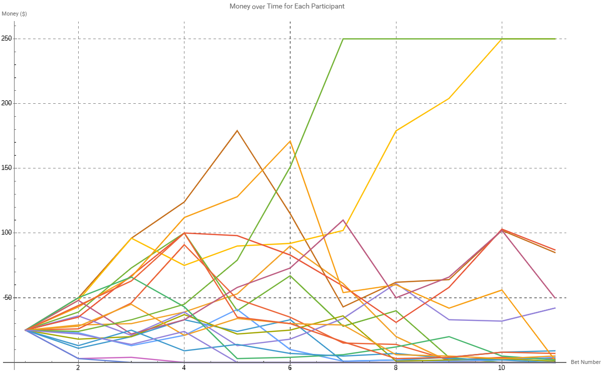
The line graph illustrates all the participants available money over time as they place bets. It can be seen that 2 of the participants have achieved $250 sum and won the game. The lower half of the graph is a bit messy. Using a heat map will better illustrate exactly what is going on.

ZeroColour[z_] := If[z == 0, Black, ColorData["Rainbow"][Rescale[z, {0.01, maxMoney}]]];
heatmapPlot = ArrayPlot[moneyResults, 
  ColorFunction -> ZeroColour,
  ColorFunctionScaling -> False,
  PlotLegends -> BarLegend[{Function[z, If[z == 0, Black, ColorData["Rainbow"][Rescale[z, {1, maxMoney}]]]],{0, maxMoney}}, 
  LegendLabel -> "Money ($)",
  LabelStyle -> {FontSize -> 12},
  Ticks -> {{0, "Broke ($0)"}, {50, "$50"}, {100, "$100"}, {150, "$150"}, {200, "$200"}, {250, "Cap ($250)"}}],
  FrameTicks -> {{Table[{i, i}, {i, numParticipants}], None}, 
                {Table[{i, i}, {i, 0, numBets}], None}},
  FrameLabel -> {{"Participant", None}, {"Bet Number", None}},
  PlotLabel -> "Money Heatmap (Black=$0)",
  ImageSize -> Large]

hitCapCount=Count[doneReasons, "Hit cap"];
wentBrokeCount=Count[doneReasons, "Went broke"];
stillPlayingCount=Count[doneReasons, "Still playing"];

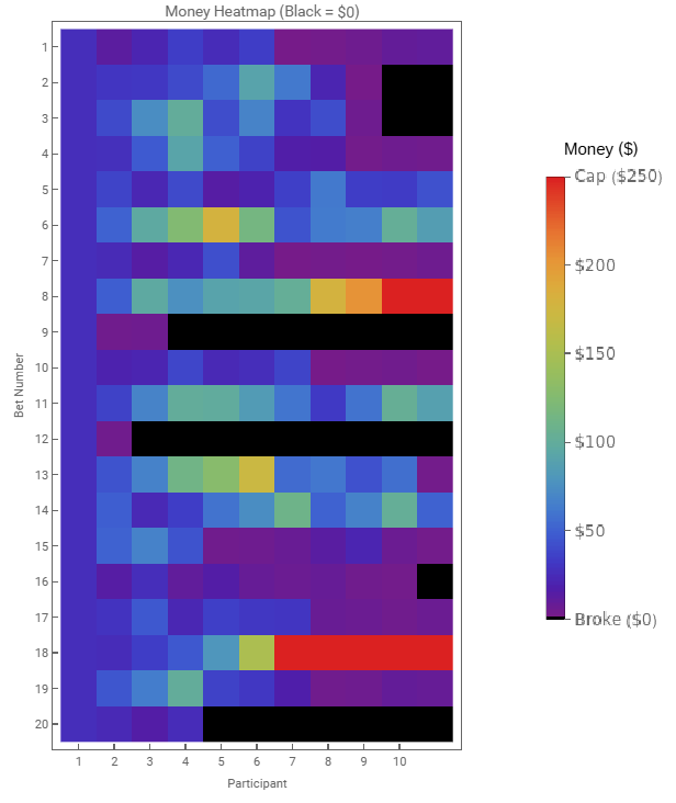
The heat map illustrates all the bets, with the black squares indicating that the participant went broke. Of the 20 participants, 6 went broke within 10 bets, or 30%, which may be surprising considering that the coin was weighted in their favour. Additionally, 8 participants ended on a purple square, suggesting a value roughly equal to or less than their starting balance. The average final balance of the participants was $39.85, a 58.7% average increase from the starting balance.

Extending to 50 Bets

Lets continue to 50 bets to see if any of the other participants are getting lucky.

numParticipants =20;
initialMoney = 25;    
numBets = 50;           
winProbability = 0.6;   
maxMoney = 250; 

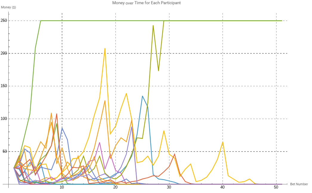
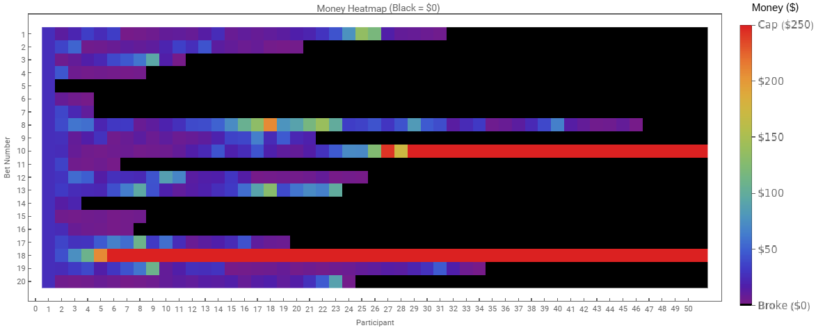
The charts reveals that only the original 2 participants who won early on in the game are winners here, with the longest playing participant ending the final losing bet at only 46 bets into the game. In the heat map it is interesting to observe that of the 6 participants who went broke within 10 bets, 4 of them (66%) went broke within the first 4 bets. The winners also appear to have accelerated quickly, with either immediate success like participant 18, or participant 10 who struggled initially and then around bet 22 saw rapid growth. It may also be deduced that there exists a survival threshold – those that managed to achieve half of the winning condition, $125, had a 25% chance of success, low but still superior odds to the 10% chance given any participant.

While these are simply observations of participants, as we increase the number of participants we can see a trend forming.

numParticipants =1000;
initialMoney = 25;    
numBets = 50;           
winProbability = 0.6;   
maxMoney = 250; 

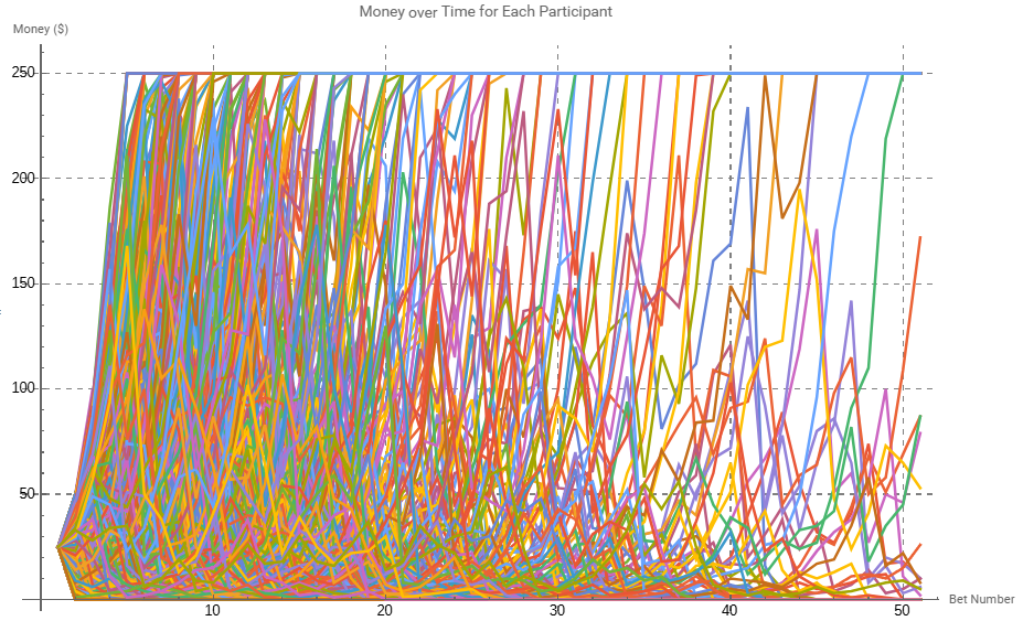
It appears that once again the majority of participants have gone broke. Another interesting observation, the aggregation of successful wagers within fewer bets, indicating a potential correlation of failure and continuous random exposure.

hitCapCount = Count[doneReasons, "Hit Cap"]
wentBrokeCount = Count[doneReasons, "Went Broke"]
stillPlayingCount = Count[doneReasons, "Still Playing"]

Of the 1000 participants, 247 successfully hit the cap, with 13 in a position of play at the end of the 50 bets. This larger test range would suggest a probability of success at 24.7%. This highlights the significance of betting size. Even with a known probability, titled in the favour of the participant, and with random betting sizes on even money bets (a somewhat oversimplification of betting on emotions or conjecture), compute ruin is not only a noteworthy concern but highly likely.

The Kelly Criterion

In probability theory, the Kelly criterion is a formula for optimising bet sizing to maximise the long term geometric growth of wealth. In systems where the return on an investment or bet is binary - that is, where one either wins or loses a fixed percentage of the wager, the expected growth rate coefficient leads to a specific optimal betting fraction.

For bets where losing the wager means losing the entire stake, the Kelly bet is given by:

$$f^*=p - \frac{q}{b} =p - \frac{1-p}{b}$$

Where: p: The probability of winning, q: The probability of losing (where q = 1-p), b: The net odds received on the wager (e.g. the amount won per unit bet if successful).

This formula determines the fraction of total wealth to bet (f*) by taking into account both the probability of winning and the payout odds. It is used to balance the potential for high returns against the risk of losing capital, ensuring that the growth of wealth is maximised over time.

The criterion works better than random even money betting because it systematically scales the bet size in relation to the bettor's edge. By focusing on maximising the expected logarithm of wealth, the strategy promotes early aggressive growth while managing risk. Logarithmic growth is key here; it reflects the compounding nature of wealth over time, where consistent, appropriately sized bets lead to a higher geometric growth rate compared to placing equal bets regardless of the edge, early gains increase your capital base, allowing subsequent bets to be more impactful.

Applying the Kelly Criterion

Applying this logic to the game, the Kelly Criterion would produce the results as follows: With even money bets (net odds b = 1) and a coin flip weighted 60% in your favour (p = 0.6), the Kelly fraction is calculated as:

$$f^* =p - \frac{1-p}{b} = 0.6 - \frac{0.4}{1}=0.2$$

This means a wager of 20% of the current bankroll.

Lets adjust the betting logic, so that each Participant applies the Kelly criterion in their betting logic. We will ensure that each bet is a whole number and a value of one or greater (as incrementally smaller amounts will theoretically result in the kelly criterion continuing bets infinitely as bet size approaches 0)

makeBet[{currentMoney_, isDone_}, winProb_, maxMoney_] := Module[{betAmount, outcome, newMoney, newIsDone, kellyFraction},
   If[isDone, Return[{currentMoney, True}]];
   If[currentMoney <=0, Return[{0, True}]];
  
   kellyFraction=2 * winProb - 1;
   
   betAmount=Floor[kellyFraction * currentMoney];
   
   If[betAmount < 1 && currentMoney > 0, betAmount = 1];
   
   outcome=RandomReal[] < winProb;
   newMoney=If[outcome, currentMoney + betAmount, currentMoney - betAmount];
   newIsDone=(newMoney>=maxMoney || newMoney <= 0);
   
   If[newMoney>=maxMoney, newMoney=maxMoney];
   If[newMoney <=0, newMoney =0];
   
   Return[{newMoney, newIsDone}]
]

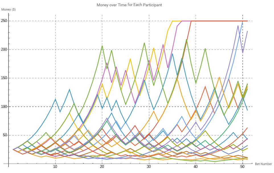
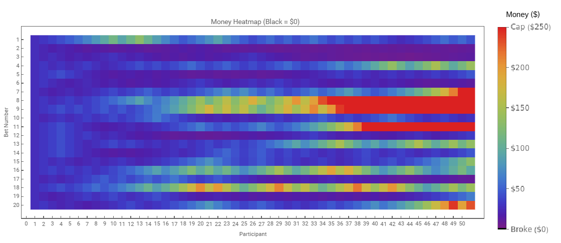
The results are remarkably different. While 4 participants reached the cap limit within 50 bets, more impressive is that not a single participant went broke. It can be observed from the line graph that more participants hold positions in the $100 - $150 range without drastic losses. Similarly, lower performing participants approaching financial ruin were able to hold positions above this point, with all but 3 making a recovery back to their original bankroll of $25. The heat map illustrates this point more clearly, with a more clearly recognisable chromatic order when approaching ruin (participant 2,3 and 17). Lets continue to 200 bets to see how the other participants perform.

numParticipants = 20;
initialMoney = 25;    
numBets = 200;           
winProbability = 0.6;   
maxMoney = 250;

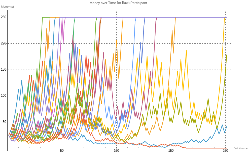
Again, the results are remarkably different from the randomly sized bets. Of the 20 participants, 17 reached the cap, representing an 85% success rate, with only 1 participant going broke within this time frame, or just 5%. It's also worth noting that the one participant that went broke did so through a gradual process, not due to a sudden significant loss. This illustrates the objective of the Kelly Criterion, maximising upward potential while preventing significant (financially ruining) downside losses.

(Side note) Notably, unlike random betting where some participants quickly reached the cap through aggressive wagering, none of the Kelly criterion users achieved the cap within the first 10 bets, (suggesting an overly conservative approach), leading some practitioners to employ double Kelly (f* x2) for faster growth. Conversely, when win probabilities are overestimated (such as believing a 60% edge when actually 55%), Kelly betting leads to ruin more frequently, prompting cautious bettors to use half Kelly (f* x0.5) as insurance. These variations lack rigorous mathematical derivation and represent practical heuristics rather than optimal mathematical solutions, and wont be discussed in detail.

Large Scale Simulation

Increasing the number of participants to 1000 reveals the following observed successes: of the 1000 participants, 852 achieved the cap (85.2%), 14 went broke (1.4%) and 134 are still in a playing position (13.4%). Besides the significantly higher success rate, it's important to recognise the amount of participants still in a position to play. Whereas the random betting left only a mere 1.3% of participants in a position to continue playing, the Kelly Criterion allows a significantly higher 13.4% to continue.

This difference highlights the Kelly Criterion's effectiveness in mitigating "gambler's ruin", the mathematical principle that predicts players with finite capital will eventually go broke against an opponent with infinite resources, regardless of the game's expected value. The Kelly strategy's conservative approach when bankrolls are small provides crucial protection against ruin by adjusting bet sizes proportionally to both bankroll and edge. This prevents the catastrophic losses that random betting strategies often produce.

The ability to remain in the game is perhaps even more important than immediate gains. Each participant who avoids ruin maintains the mathematical possibility of future success, preserving their option value. This persistence advantage compounds over time, as those still playing have the opportunity to experience positive variance and potentially reach the maximum.

Conclusion

This study compared random even money betting with the Kelly criterion betting strategy across multiple simulated participants. The objective was to demonstrate how mathematical optimisation in betting can lead to dramatically different outcomes compared to arbitrary bet sizing. The results demonstrate the Kelly criterion's remarkable effectiveness: 85% of participants reached the capital cap versus only a small percentage with random betting. Most importantly, while random betting left only 1.3% of participants able to continue playing, Kelly betting preserved 13.4% of participants in addition to those who reached the cap.

The Kelly formula has a significant limitation in real world applications; it assumes perfect knowledge of probabilities, which is rarely available in actual gambling or financial markets. When probabilities are misestimated (believing you have a 60% edge when it's actually 55%), the formula can lead to unexpected ruin, and this has been thoroughly criticised by gamblers and cryptocurrency "investors" alike. This study highlights the critical importance of proper bet sizing and consideration of gambler's ruin, the mathematical certainty that players with finite capital will eventually go broke against an opponent with infinite resources, even when odds are favourable. Kelly betting demonstrates how mathematical principles can protect against this outcome through strategic capital allocation.

A point for further analysis would be exploring the applications of the Kelly criterion as a risk management tool. Beyond the context of gambling, decisions often reflect binary outcomes with limited information, effectively even money bets with estimated winning probabilities. Decisions may be modelled as bets, balancing aggressive pursuit of advantage against protection from ruin, addressing the challenge of all risk management, recourse planning and project management, how to capture upside potential without exposing the enterprise to financial ruin, and to keep playing. Thanks for reading.

Attachments:

KellyCritEvenMoney.nb