When designing industrial processes, physics is just one piece of the puzzle. We often create models to simulate fluid flow or thermal behavior. But what happens when we need to integrate discrete control logic—especially for multi-step systems like batch processes?

This is where things get tricky. You might have a solid physical model, but no clear way to simulate real-world automation behavior—like timed valve switching, temperature-based triggers, or pump sequencing.

In this example, I’ll walk you through how to bridge that gap by combining physical modeling—like fluid flow and heat transfer—with event-driven logic using Statecharts to replicate an automated batch process.

Whether you’re working in pharmaceuticals, chemical manufacturing, or food processing, this workflow lets you simulate and test control strategies before deploying them. That means fewer manual errors, faster iterations, and a complete view of the process—all in one unified model.

Step 1: Build the Fluid System

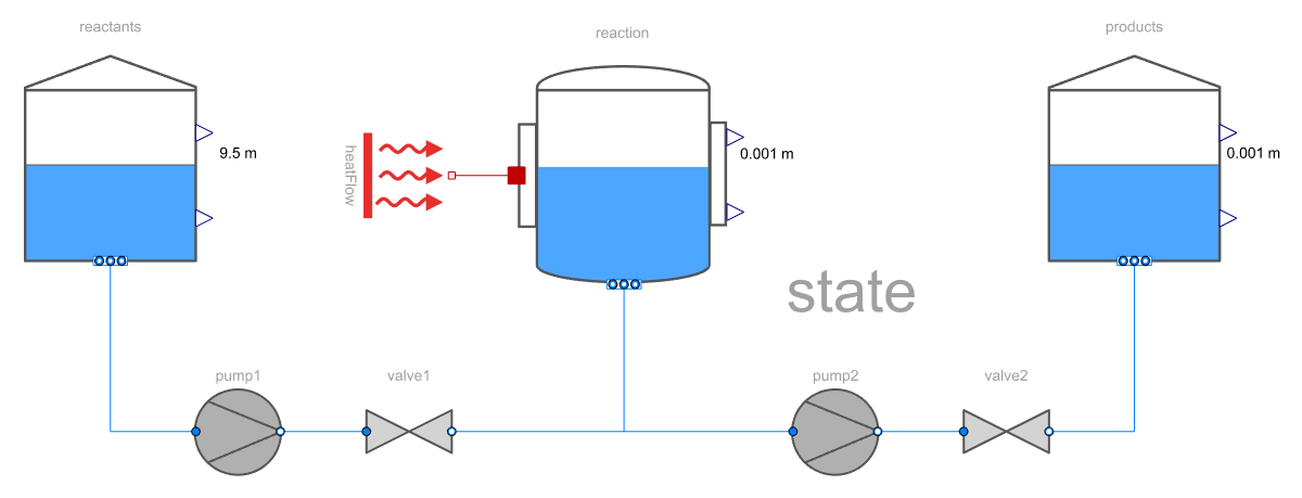
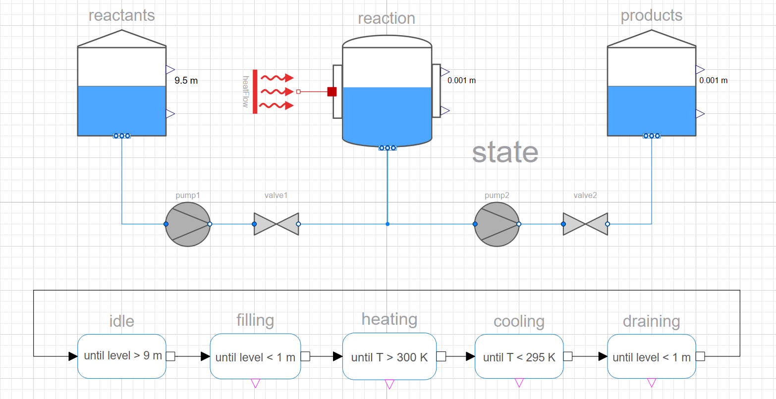
We start by designing a fluid circuit that mirrors the real-world process. The system has three tanks:

• A reactant tank to store the raw input,
• A reaction tank where heating or cooling takes place, and
• A product tank to collect the output.

The reaction tank is equipped with a heater/cooler that we can control externally.

Using the Modelica Fluid library, I assembled this system with built-in components like tanks, pumps, and valves. These components capture essential behavior—flow dynamics, temperature changes, and pressure effects—and I could just connect them without needing to enforce conservation laws manually (that’s the power of acausal modeling).

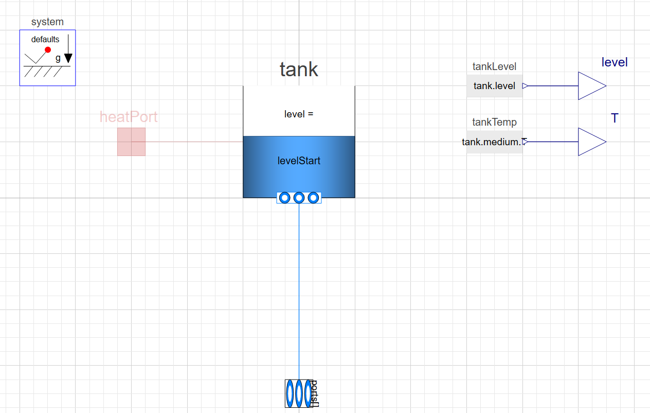
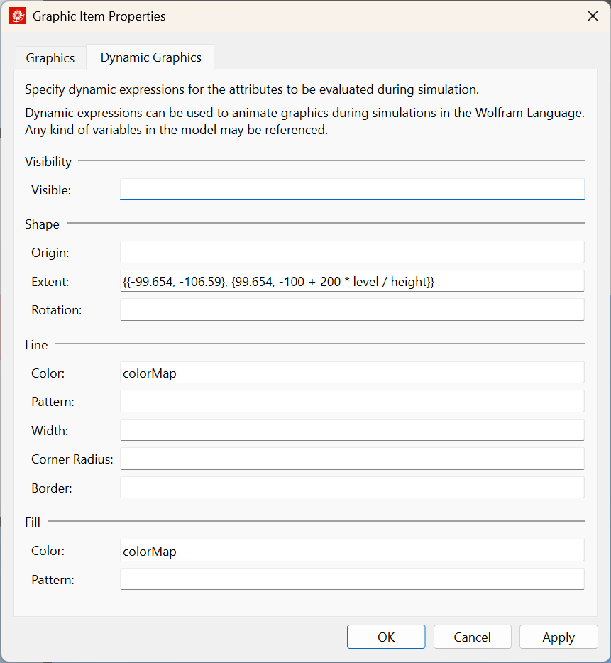
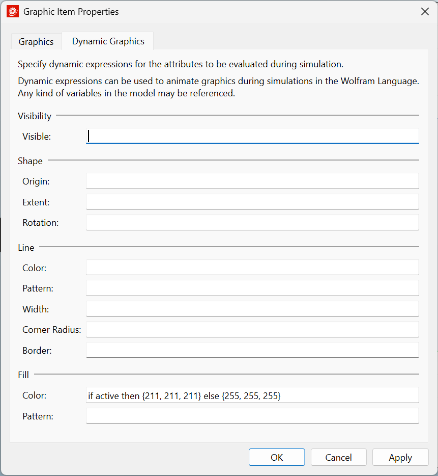
To make the simulation more intuitive, I added dynamic visuals. For example, tank levels update in real time, and fluid color reflects temperature, making it easier to understand the system at a glance.

Step 2: Define the Event Logic with Statecharts

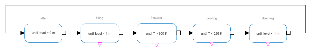
Next, we define the control logic with a state machine using the Modelica StateGraph library. Here’s the basic sequence:

• The system starts in an Idle state.
• After 5 seconds, it transitions to Filling, where the reaction tank fills with reactant.
• Once the level reaches 9 meters (reaction tank), it switches to Heating.
• When the temperature hits 300 K, we move to Cooling.
• Cooling continues until the temperature drops to 295 K, triggering the Draining state.

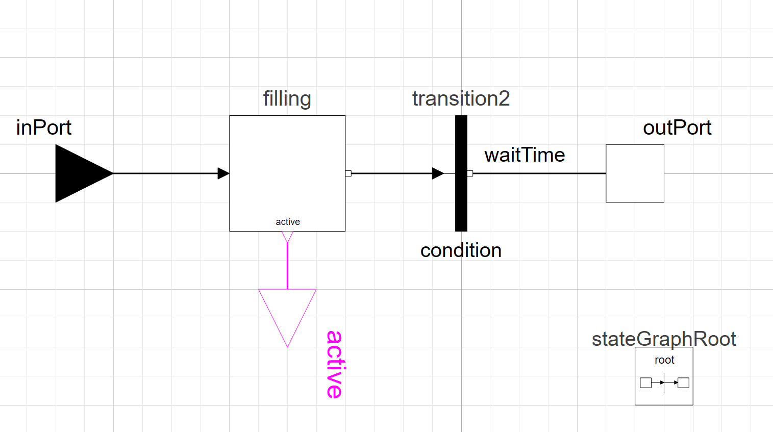
Each of these transitions is based on time or sensor feedback (using conditional events). I also added visual indicators to the icons, so you can immediately see which state is active during simulation.

Step 3: Couple the State Machine with the Physical Model

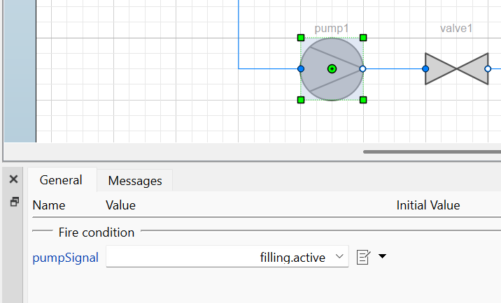
Now we connect the submodels. The fluid components contain boolean signal inputs that gets triggered based on the state machine. The state machine controls the physical system by:

• Opening and closing valves,
• Activating the heater,
• Starting and stopping the pump.

This hybrid approach—discrete control logic layered on top of a fluid model—closely mirrors how real industrial automation systems operate.

Visualizing the Results

I ran the simulation in Wolfram Language and created an animation to help visualize the entire process flow. You can see how fluid moves, how temperature changes, and how the control logic reacts in sync.

You can download the full model and the notebook used for the animation here: Batch Process Example

Want to learn more about fluid modeling in System Modeler? Check out this guide: Getting Started with Fluid Modeling

Have a specific process in mind? Drop it in the comments—I’d love to hear about it.