Comments on the post: Photon propagation through variable-dimensional space
We can think of the path of engineering innovation in the Game of Life as like an effort to navigate through an ocean of computational irreducibility, finding islands of reducibility. That island mentality, reflects a bit of a "time out" diffraction, of Bessel functions to describe radial wave solutions and gravitational potentials in fractional-dimensional space. These mathematical functions have a very lucky solution; it's like the "catfish" of trigonometric scenarios; structured solutions emerge in seemingly chaotic environments.
ClearAll["Global`*"];
FractionalBesselJ[\[Nu]_, r_] := (r)^((3 - D)/2)*BesselJ[\[Nu], r]
PotentialSolution[D_, r_, z_, k_] :=
 Module[{\[Nu], radialPart, verticalPart}, \[Nu] = (D - 3)/2;
  radialPart = FractionalBesselJ[\[Nu], k*r];
  verticalPart = Exp[-k*Abs[z]];
  radialPart*verticalPart]
kValue = 0.1;
DValues = {2.0, 2.5, 3.0};
plots = Table[
   Plot3D[Evaluate[
     PotentialSolution[D, Sqrt[x^2 + y^2], 0, kValue]], {x, -30,
     30}, {y, -30, 30}, PlotRange -> All,
    PlotLabel -> StringForm["D=``", D],
    ColorFunction -> "TemperatureMap",
    AxesLabel -> {"X", "Y", "Potential"},
    BoxRatios -> {1, 1, 0.7}], {D, DValues}];
Grid[Partition[plots, 3], Spacings -> {0, 0}]
CircularVelocity[D_, r_?NumericQ] :=
 Module[{\[Nu], k, integral}, \[Nu] = (D - 3)/2;
  k = 1/r;
  integral =
   NIntegrate[k^((3 - D)/2)*BesselJ[\[Nu], k*r]*k^(D/2), {k, 0, 1},
    Method -> "GlobalAdaptive"];
  Sqrt[Abs[integral*r]]]
velocityPlot =
 Plot[Evaluate[Table[CircularVelocity[D, r], {D, {2.5, 3.0}}]], {r, 1,
    30}, PlotStyle -> {Red, Blue},
  PlotLegends -> {"D=2.5", "Newtonian (D=3)"},
  AxesLabel -> {"Radius", "Circular Velocity"},
  PlotLabel -> "Rotation Curve Comparison"]
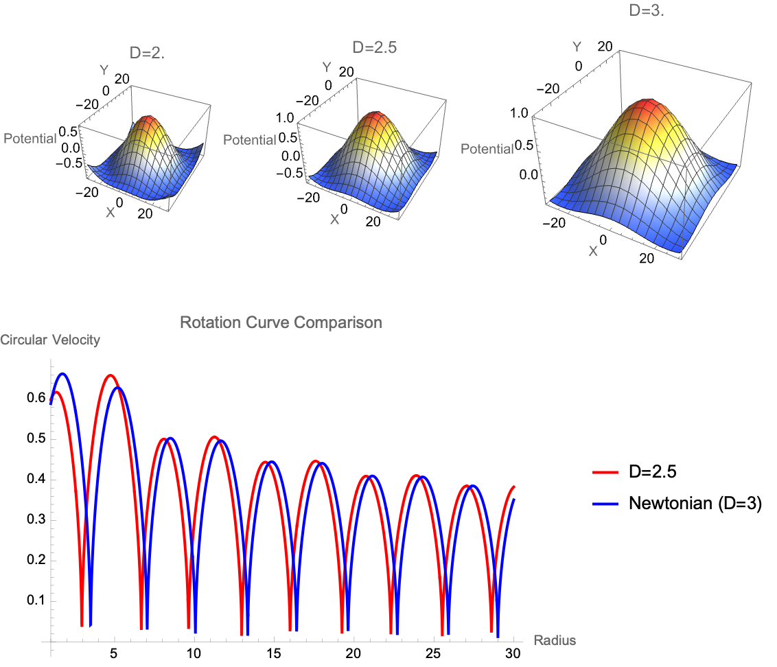
It's a lucky solution, structured Bessel functions are analogous to stable "islands" within irreducible mathematical complexity. But most of the time, the first step is to identify an objective, some purpose one can describe and wants to achieve. Here, instead of the new mayor in town we can revert to the old, simulation of circular velocities and rotation curves which are critical in astrophysics..the computational objective, is defined and "geared" towards structures like gliders which serve defined purposes in cellular automata, engineering goals. Velocity curves are purposefully and "intentionally" measured for the purpose of paralleling structured engineering in "Conway's Game of Life".
ClearAll[potential];
potential[R_, z_, D_, k_] := (k*R)^((3 - D)/2)*
  BesselJ[(D - 3)/2, k*R]*Exp[-k*Abs[z]]
DValue = 2.5;
kValue = 1;
Plot3D[potential[R, z, DValue, kValue], {R, 0.1, 5}, {z, -5, 5},
 PlotRange -> All,
 AxesLabel -> {"R", "z", "Potential \[CapitalPhi](R,z)"},
 PlotLabel ->
  Style["Fractional-Dimensional Potential (D = " <> ToString[DValue] <>
     ")", 14, Bold], ColorFunction -> "TemperatureMap",
 MeshFunctions -> {#3 &}, MeshStyle -> Opacity[0.3],
 ImageSize -> 600]
ContourPlot[potential[R, z, DValue, kValue], {R, 0.1, 5}, {z, -5, 5},
 FrameLabel -> {"R", "z"},
 PlotLabel ->
  Style["Equipotential Contours (D = " <> ToString[DValue] <> ")", 14,
    Bold], ColorFunction -> "TemperatureMap", Contours -> 20,
 ImageSize -> 600]
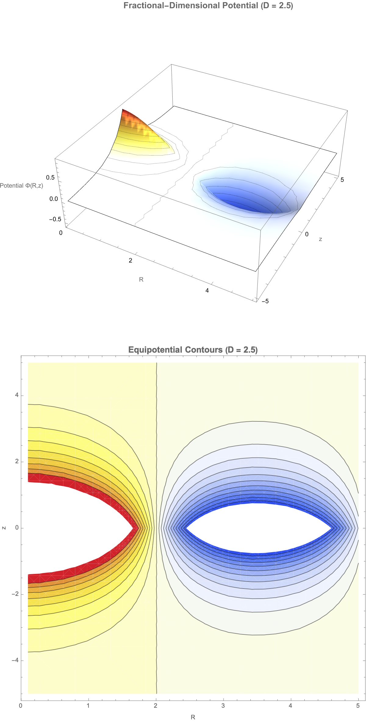
The K-night, this is the same thing that we took in, it's fractional cylindrical Laplacian engineering--whatever raw material is available..fashion it into something that aligns with human purposes. The fractional cylindrical Laplacian represents how fractional dimensions, Bessel functions, cylindrical coordinates (mathematical "raw materials") are fashioned to achieve named and defined objectives--solving wave equations in non-integer dimensions, basic mathematical "materials" show and represent the purposeful manipulation of complexity via the structural way that the Game of Life, its rivers cross in structurally unexpected and fun ways.
FractionalCylindricalLaplacian[\[Psi]_, R_, \[Phi]_,
  z_, \[Alpha]R_, \[Alpha]\[Phi]_, \[Alpha]z_] :=
 Module[{Dtotal = \[Alpha]R + \[Alpha]\[Phi] + \[Alpha]z}, (1/
      R^(Dtotal - 2)*
     D[R^(Dtotal - 2)*D[\[Psi], R],
      R] + (1/(R^2*Sin[\[Phi]]^(Dtotal - 3)))*
     D[Sin[\[Phi]]^(Dtotal - 3)*D[\[Psi], \[Phi]], \[Phi]] + (1/
       z^(\[Alpha]z - 1))*D[z^(\[Alpha]z - 1)*D[\[Psi], z], z])]
FractionalCylindricalWaveSolution[R_, \[Phi]_, z_, k_, m_,
  Dtotal_, \[Alpha]R_, \[Alpha]\[Phi]_, \[Alpha]z_] :=
 Module[{\[Lambda] = (Dtotal - 3)/2, radialSolution, angularSolution,
   zSolution},
  radialSolution = (k*R)^((3 - Dtotal)/2)*
    BesselJ[(Dtotal - 3)/2 + m, k*R];
  angularSolution = GegenbauerC[m, \[Lambda], Cos[\[Phi]]];
  zSolution = Exp[-k*Abs[z]];
  radialSolution*angularSolution*zSolution]
Module[{M = 1.5*10^41, g\[Dagger] = 1.2*10^-10, G = 6.674*10^-11, l0,
  Rd, wd, kValues, Dtotal = 1.7, results}, l0 = Sqrt[G*M/g\[Dagger]];
 Rd = 30000*9.461 e15; wd = Rd/l0;
 kValues = Subdivide[0.1, 2.0, 50];
 results =
  Table[FractionalCylindricalWaveSolution[R, 0, 0, k, 0, Dtotal, 1, 1,
     1], {k, kValues}, {R, 0.1*l0, 5*l0, l0/10}];
 DensityPlot3D[
  FractionalCylindricalWaveSolution[Sqrt[x^2 + y^2], ArcTan[y/x], z,
   0.1, 0, Dtotal, 1, 1, 1], {x, -l0, l0}, {y, -l0, l0}, {z, -l0/10,
   l0/10}, PlotRange -> All, ColorFunction -> "TemperatureMap",
  AxesLabel -> {"X (m)", "Y (m)", "Z (m)"},
  PlotLabel -> "Fractional-Dimensional Gravitational Potential"]]
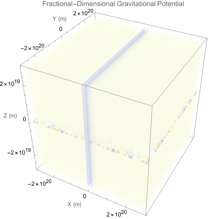
Why fractional? Well, it's like..a "rough" analogy would be the film North by Northwest, you just keep ordering cupcakes and whatever and it just becomes totally disgusting, but those are the delicatessens that show how, we Ruliologically engineer solutions to wave forms from fractional-dimensional equations. And, they don't simply occur "scientifically" or nationally, you just keep getting iterations and various issues with those iterations until you reach, the intentional creation and natural constraints that occur within the realm of computationally purposeful, engineered patterns in cellular automata. But hopefully we can get more action than that. Hopefully we can carefully construct patterns, not random occurrences, the closest next of kin which would be the constructed cellular automaton configurations.
ClearAll["Global`*"];
radialSolution[R_, k_, D_] := (k*R)^((3 - D)/2)*BesselJ[(D - 3)/2, k*R]
potential[R_, z_, D_, k_] :=
 Module[{angularPart, radialPart, zPart}, angularPart = 1;
  radialPart = radialSolution[R, k, D];
  zPart = Exp[-k*Abs[z]]; radialPart*angularPart*zPart]
DValue = 2.5;
kValue = 0.1;
potentialField =
  Table[{R, z, potential[R, z, DValue, kValue]}, {R, 0.1, 10,
    0.1}, {z, -5, 5, 0.1}];
potentialFieldFlat = Flatten[potentialField, 1];
ListPlot3D[potentialFieldFlat,
 AxesLabel -> {"R (kpc)", "z (kpc)", "Potential \[CapitalPhi](R,z)"},
 PlotLabel ->
  Style["Fractional-Dimensional Potential (D=" <> ToString[DValue] <>
    ")", 16, Bold], ColorFunction -> "TemperatureMap",
 PlotRange -> All, Mesh -> None, PlotLegends -> BarLegend[Automatic],
 ImageSize -> Large, BoxRatios -> {1, 1, 0.5}]
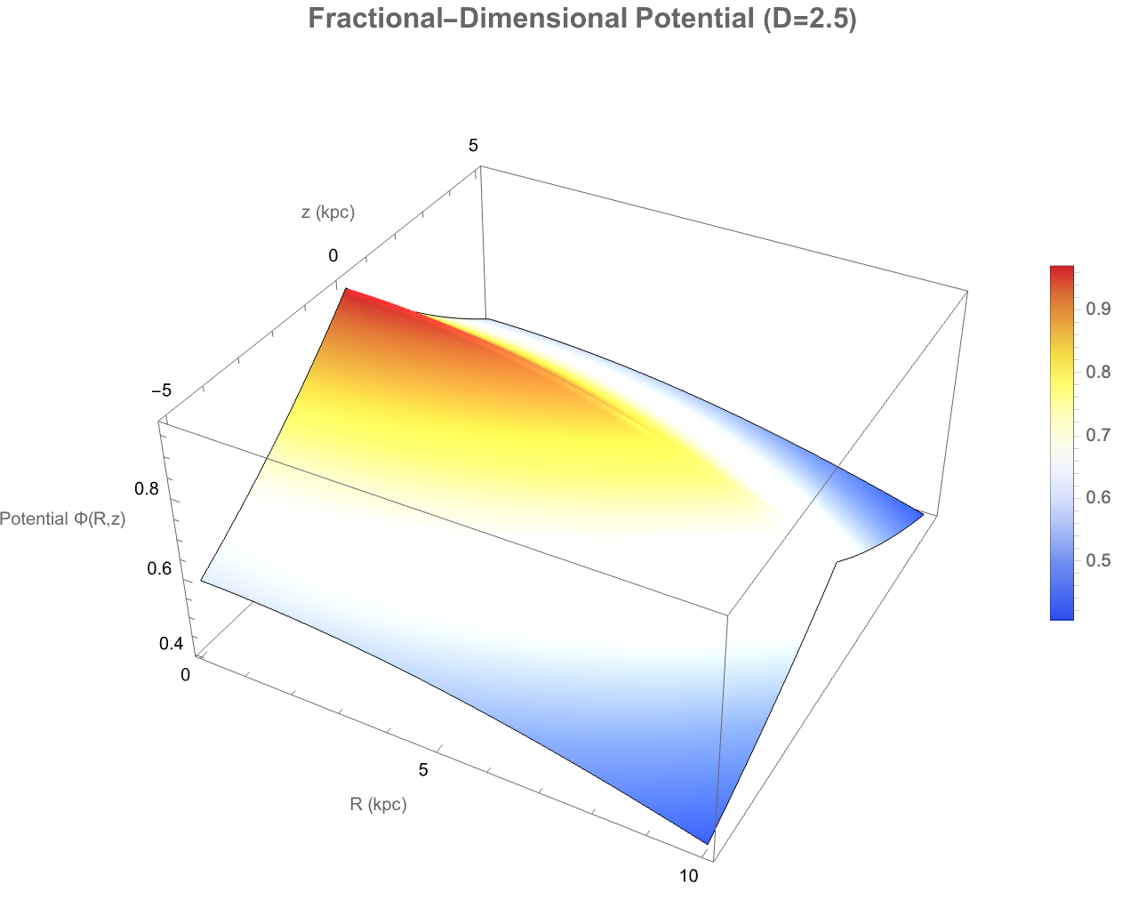
You can see the blocks and "Eaters", you can see the density plots and contour plots that's, if we want to get closer to the study of the pure phenomenon of innovation..everything that happens can be described in a uniform way. "The closest thing we have to a Hilbert space" is, with the standardization of complex solutions into "pretty" uniform, understandable forms, we get clear, human-readable configurations--much like visualizing automaton patterns for "better" understanding. With the snap of a finger, the reduction of computational complexity becomes relevantly reduced into a form that is analogous to the evolution of automaton states.
ClearAll["Global`*"];
\[Alpha]1 = 0.5;
\[Alpha]2 = 0.5;
\[Alpha]3 = 1.0;
Ddim = \[Alpha]1 + \[Alpha]2 + \[Alpha]3;
m = 0;
\[Beta]\[Rho] = 1.0;
\[Beta]z = 1.0;
\[Nu] = 0.5*Sqrt[(2 - \[Alpha]1 - \[Alpha]2)^2 + 4*m^2];
f[\[Rho]_] := \[Rho]^((1 - (\[Alpha]1 + \[Alpha]2)/
2))*(BesselJ[\[Nu], \[Beta]\[Rho]*\[Rho]] +
BesselY[\[Nu], \[Beta]\[Rho]*\[Rho]]);
A = 0; B = 0;
c = (2 - \[Alpha]2)/2;
\[Xi][\[Phi]_] := Sin[\[Phi]]^2;
g[\[Phi]_] :=
Hypergeometric2F1[A, B, c, \[Xi][\[Phi]]] + \[Xi][\[Phi]]^(1 - c)*
Hypergeometric2F1[A - c + 1, B - c + 1, 2 - c, \[Xi][\[Phi]]];
n = 1 - \[Alpha]3/2;
h[z_] := z^n*(BesselJ[n, \[Beta]z*z] + BesselY[n, \[Beta]z*z]);
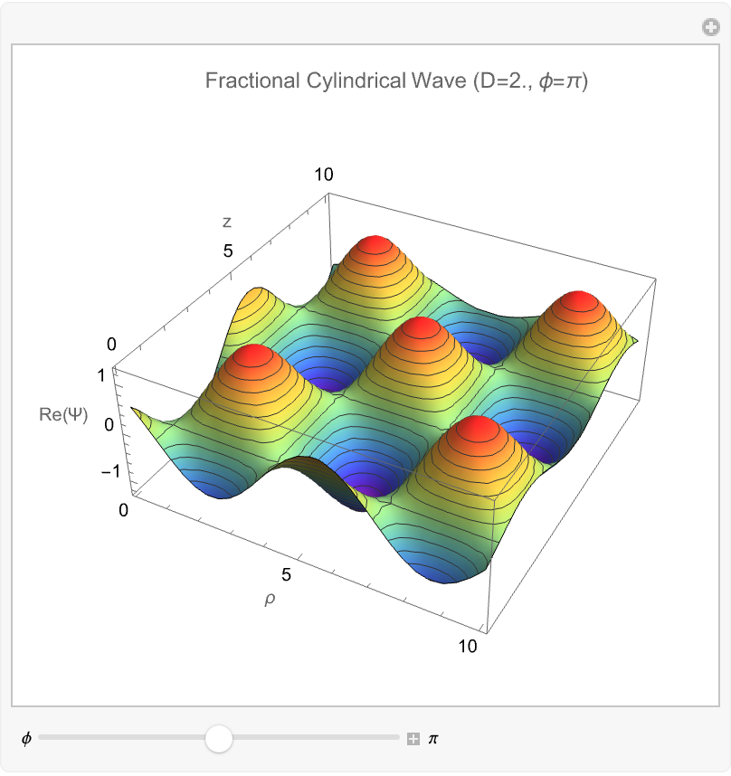
\[CapitalPsi][\[Rho]_, \[Phi]_, z_] := f[\[Rho]]*g[\[Phi]]*h[z];
Manipulate[
Plot3D[Re[\[CapitalPsi][\[Rho], CurlyPhi, z]], {\[Rho], 0.1, 10}, {z,
0.1, 10}, PlotRange -> All,
AxesLabel -> {"\[Rho]", "z", "Re(\[CapitalPsi])"},
PlotLabel ->
StringForm["Fractional Cylindrical Wave (D=``, \[Phi]=``)", Ddim,
CurlyPhi], ColorFunction -> "Rainbow", MeshFunctions -> {#3 &},
PerformanceGoal -> "Quality"], {{CurlyPhi, \[Pi], "\[Phi]"}, 0,
2 \[Pi], \[Pi]/10, Appearance -> "Labeled"},
ControlPlacement -> Bottom]
A typical manifestation of computational irreducibility, many small and seemingly random looking symmetries..results were "found". Fractional-dimensional gravitational potentials and field simulations sometimes started to appear : an important methodology, has revolved around so-called hasslers providing harnesses that rein in behavior. The gravitational potentials and fields, "being" complex, computationally irreducible phenomena that are effectively "harnessed" and viewed through these mathematical functions and simulations, "just as" hasslers rein in chaotic automaton behavior, in fact out of the corner of our simulation, here instead I think Simon Fischer our audience might be able to understand..engineered control in cellular automata, via the careful analysis and constraints..of behaviorally complex gravitational fields.
ClearAll["Global`*"];
DValue = 2.5;
m = 0;
k = 1;
Rd = 0.681;
RadialSolution[R_] := (k*R)^((3 - DValue)/2)*
  BesselJ[(DValue - 3)/2 + m, k*R]
AngularSolution[\[Phi]_] := GegenbauerC[m, (DValue - 3)/2, Cos[\[Phi]]]
Psi[R_, \[Phi]_] := RadialSolution[R]*AngularSolution[\[Phi]]
DensityPlot[
 Psi[Sqrt[x^2 + y^2], ArcTan[x, y]], {x, -5, 5}, {y, -5, 5},
 ColorFunction -> "SunsetColors", PlotLegends -> BarLegend[Automatic],
  FrameLabel -> {"X (kpc)", "Y (kpc)"},
 PlotLabel -> StringForm["Fractional Potential (D = ``)", DValue],
 PlotRange -> All, Exclusions -> None, PlotPoints -> 100,
 ImageSize -> Large]
If[DValue > 2,
 Plot3D[Psi[Sqrt[x^2 + y^2], ArcTan[x, y]], {x, -5, 5}, {y, -5, 5},
  ColorFunction -> "SunsetColors",
  PlotLabel -> StringForm["3D Potential View (D = ``)", DValue],
  AxesLabel -> {"X", "Y", "\[CapitalPsi]"}, PlotRange -> All,
  Exclusions -> None, PlotPoints -> 50, BoxRatios -> {1, 1, 0.5},
  ImageSize -> Large]]
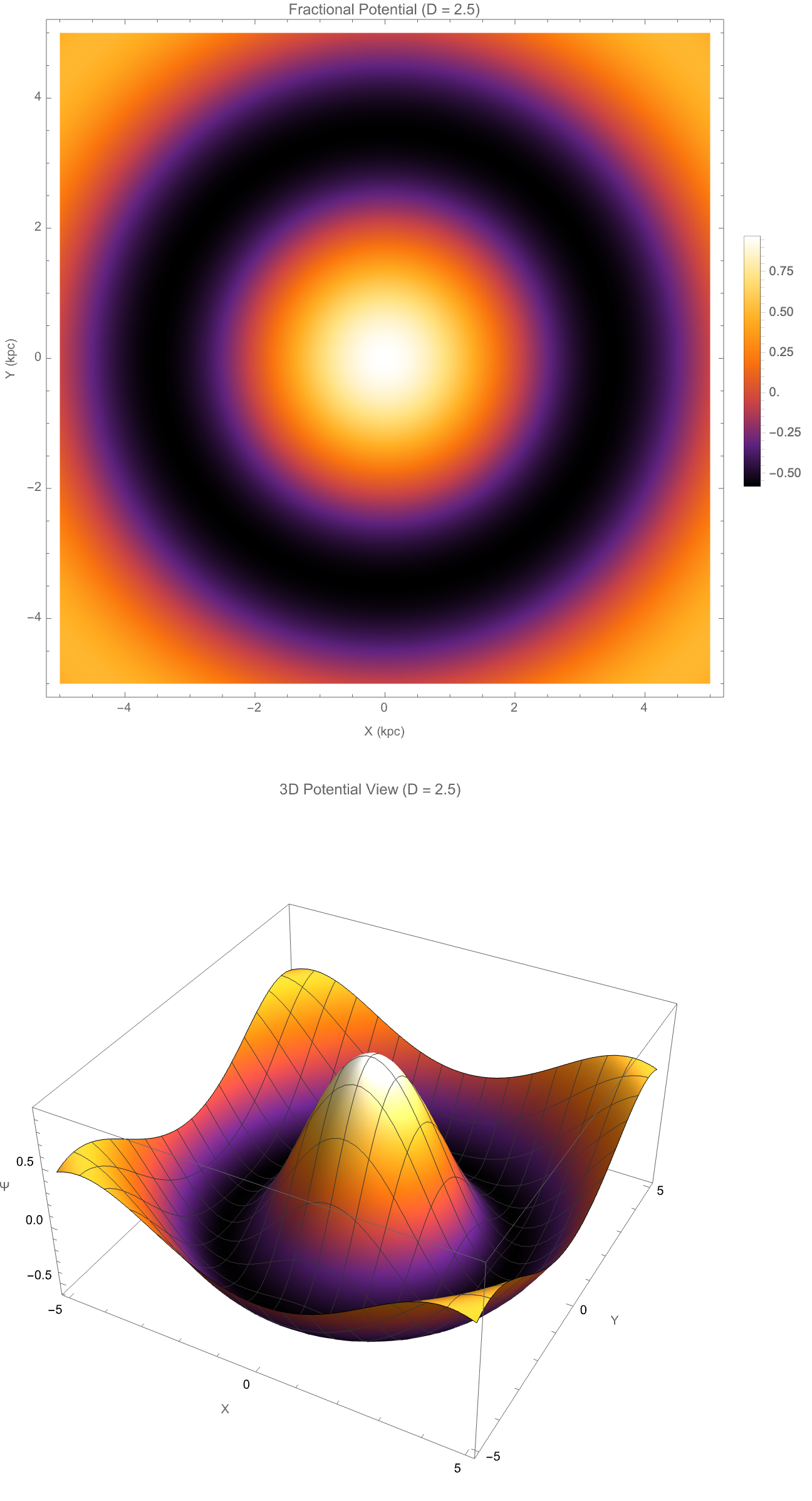
With regard to these "isomorphisms"..cylindrical wave functions with Gegenbauer polynomials and "hypergeometric" functions, it's a beautiful thing; one theme to which we'll return later is that after certain functionality was first built, many optimizations achieving that functionality more robustly, exist, and the sophisticated mathematical constructs like Gegenbauer polynomials climb out of the picturesque, optimized solutions to fractional-dimensional problems, and that is where we get our improved, engineered automaton solutions from initial "complicated" constructions to simpler, optimized versions. The mathematically "optimized" formulation demonstrates engineered improvements.
ClearAll["Global`*"];
dim = 2.5;
radialTerm[\[Phi]_, R_, z_] :=
D[\[Phi][R, z], {R, 2}] + (dim - 2)/R*D[\[Phi][R, z], R];
angularTerm[\[Phi]_, R_, z_] := 0;
verticalTerm[\[Phi]_, R_, z_] := D[\[Phi][R, z], {z, 2}];
fractionalLaplacian[\[Phi]_, R_, z_] :=
radialTerm[\[Phi], R, z] + angularTerm[\[Phi], R, z] +
verticalTerm[\[Phi], R, z] == 0;
\[Phi][R_, z_] := J[R] Z[z];
k = 1;
Z[z_] := Exp[-k Abs[z]];
reducedEquation =
fractionalLaplacian[\[Phi], R, z] /. Z[z] -> Exp[-k Abs[z]];
reducedRadialEquation =
Simplify[reducedEquation,
Assumptions -> {R > 0, z \[Element] Reals, k > 0}] /. J[R] -> j[R];
radialSolution = DSolve[reducedRadialEquation, j[R], R] // Simplify;
generalSolution = \[Phi][R, z] -> (j[R] /. radialSolution[[1]]) Z[z];
TraditionalForm[generalSolution]
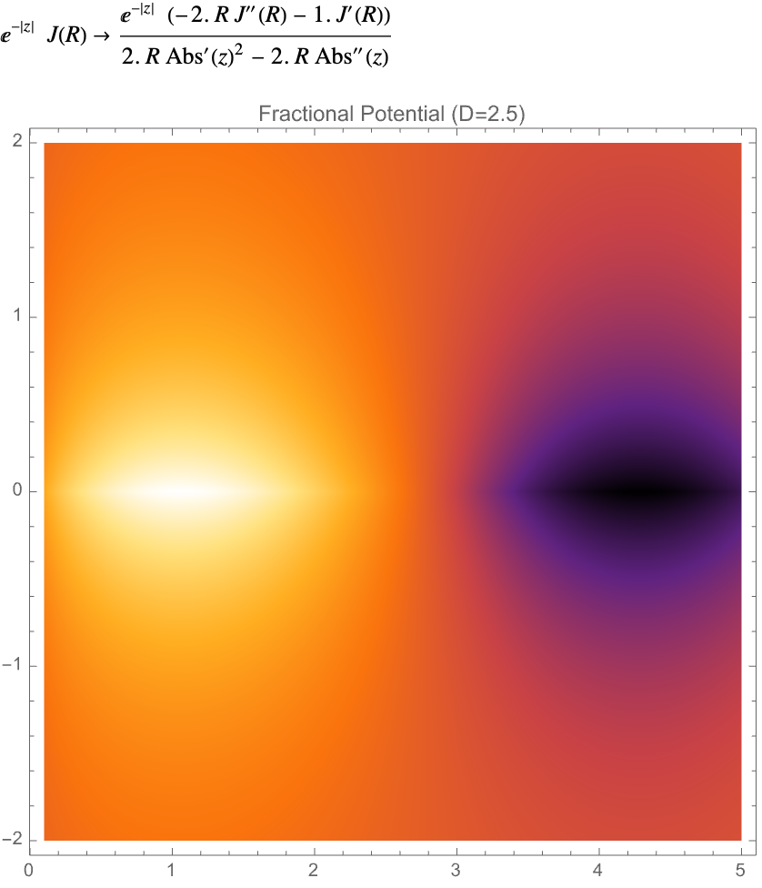
radialFunction[R_] :=
R^((3 - dim)/2)*(BesselJ[(dim - 3)/2, k R] +
BesselY[(dim - 3)/2, k R]);
DensityPlot[
radialFunction[R]*Exp[-k Abs[z]] /. {k -> 1}, {R, 0.1, 5}, {z, -2,
2}, PlotLabel -> "Fractional Potential (D=2.5)",
AxesLabel -> {"R", "z"}, ColorFunction -> "SunsetColors",
PlotRange -> All, PlotPoints -> 100, ImageSize -> Large]
And it's not, Wolfram Community's fault that I can't, for instance, put brackets, I can't put back slashes \ "behind" or in front of the image name.. somewhere along the way, the Wolfram, the computational irreducibility is the spark in the system. The cage provides the control we need. That's right, these Partial Differential Equations, Fractional-Dimensional represent, computationally irreducible equations where, boundary conditions or cages ("constraints") allow structured solutions, which "at least" mirror, how chaotic behavior in automata is controlled for purposeful engineering. So the real complexity is the file system..complexity here is "caged" by boundary conditions to yield structured solutions.
ClearAll["Global`*"];
FractionalCylindricalLaplacian[\[Phi]_, R_, z_, D_] :=
D[\[Phi], {R, 2}] + (D - 2)/R D[\[Phi], R] + D[\[Phi], {z, 2}];
RadialSolution[D_, k_,
R_] := (k R)^((3 - D)/2) BesselJ[(D - 3)/2, k R];
ZSolution[k_, z_] := Exp[-k Abs[z]];
FractionalPotential[R_, z_, D_, k_] :=
RadialSolution[D, k, R]*ZSolution[k, z];
DValue = 2.5;
kValue = 1;
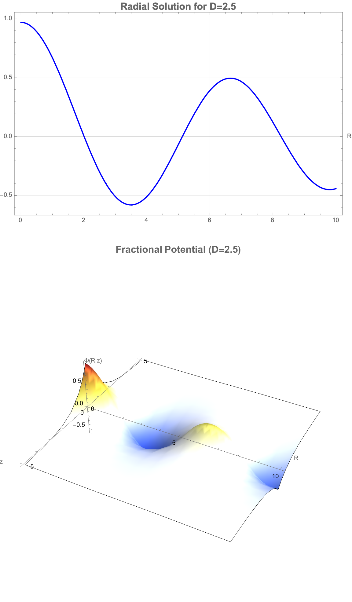
Plot[RadialSolution[DValue, kValue, R], {R, 0, 10},
PlotLabel ->
Style["Radial Solution for D=" <> ToString[DValue], 16, Bold],
AxesLabel -> {"R", "J(R)"}, PlotStyle -> {Thick, Blue},
GridLines -> Automatic, Frame -> True, ImageSize -> Large]
Plot3D[FractionalPotential[R, z, DValue, kValue], {R, 0.1,
10}, {z, -5, 5},
PlotLabel ->
Style["Fractional Potential (D=" <> ToString[DValue] <> ")", 16,
Bold], AxesLabel -> {"R", "z", "\[CapitalPhi](R,z)"},
ColorFunction -> "TemperatureMap", PlotRange -> All, Mesh -> None,
Boxed -> False, AxesOrigin -> {0, 0, 0}, ImageSize -> Large]
How did we do that? In the parametric and modular approach (it's a non-sequitur), the main emphasis tends to be on figuring out plans, then constructing things based on those plans. These, we have seen enough of the modular approach. Forget the modular approach. Personally, I would rather mirror structured engineering methods, where plans or oscillators, gliders, and guns in automata (modules) are systematically combined. It is systematic, engineered construction that is analogous to modular engineering in automata: parametric modules and Manipulate make it possible to engage in "building from history".
ClearAll["Global`*"];
RadialSolutionD[R_, k_, D_, m_] := (k*R)^((3 - D)/2)*
  BesselJ[(D - 3)/2 + m, k*R]
m = 0;
k = 1;
DValues = {2.0, 2.5, 3.0};
colorList = {Red, Green, Blue, Purple, Orange};
radialPlots =
  Table[Plot[RadialSolutionD[r, k, Dval, m], {r, 0.1, 10},
    PlotRange -> All,
    PlotLabel ->
     Style["Radial Solution for D = " <> ToString[Dval], 14, Bold],
    AxesLabel -> {"R", "J(R)"}, PlotStyle -> {Thick, colorList[[i]]},
    ImageSize -> {360, 360}, Frame -> True, GridLines -> Automatic,
    GridLinesStyle -> Directive[Gray, Dashed],
    AspectRatio -> 1/GoldenRatio], {Dval, DValues}, {i,
    Length[DValues]}];
GraphicsGrid[Partition[radialPlots, 2], Frame -> All,
 FrameStyle -> LightGray, Spacings -> {2, 2},
 Background -> Lighter[Gray, 0.95], ImageSize -> 800]
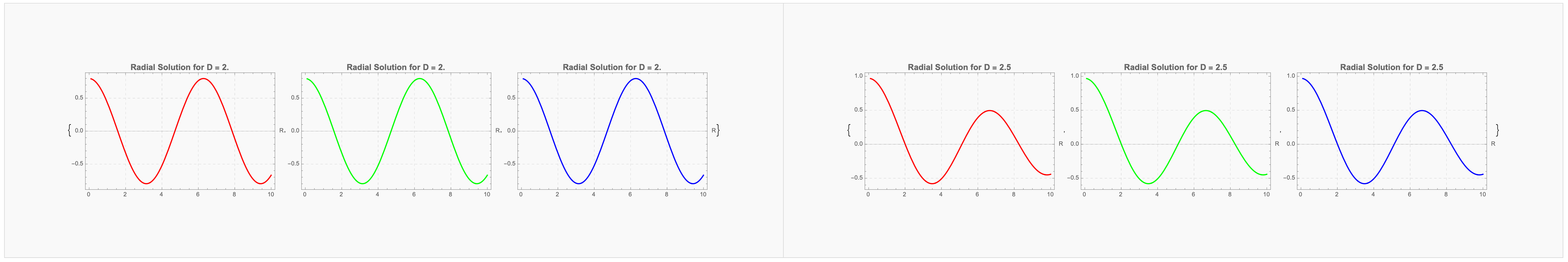
Via causal graphs and computational irreducibility, causal graphs are much more revealing. They show that there are lots of factored modular parts or irreducible blobs; although causal graphs are couched in structured solutions that reflect attempts to isolate "modular parts" or "irreducible blobs" through mathematical analysis much like analyzing structures in cellular automata. Sure, we can "extend" our..complex fractional solutions to implicitly explore irreducibility versus modularity--similar to how causal graphs differentiate modular (engineering) from chaotic (pure computational irreducibility). With a roll of the dice, we can computationally meta-engineer concepts from the Game of Life by harnessing complexity and 'achieving well-defined objectives', optimizing modularity, as well as the irreducible phenomena that we clarify visually, parametrically "explore" the creative engineering methodologies described, particularly the duality of structured plans versus computational exploration.
Manipulate[
 Module[{potential, R, z},
  potential[R_, z_] = (k R)^((3 - D)/2)*BesselJ[(D - 3)/2, k R]*
    Exp[-k Abs[z]];
  Plot3D[potential[r, zz], {r, 0, 5}, {zz, -5, 5}, PlotRange -> All,
   ColorFunction -> (ColorData["TemperatureMap"][#3] &),
   MeshFunctions -> {#3 &},
   AxesLabel -> {"R", "z", "\[CapitalPhi](R,z)"},
   PlotLabel ->
    Style[Row[{"Fractional-Dimensional Potential\n", "D = ",
       NumberForm[D, {3, 1}], ",  k = ", NumberForm[k, {3, 1}]}], 14,
     Bold], BoxRatios -> {1, 1, 0.6},
   PerformanceGoal -> "Quality"]], {{D, 2.5, "Dimension"}, 2, 3, 0.1,
  Appearance -> "Labeled",
  ImageSize -> Small}, {{k, 1.0, "Wave Number"}, 0.1, 2, 0.1,
  Appearance -> "Labeled", ImageSize -> Small},
 ControlPlacement -> Left, TrackedSymbols :> {D, k},
 FrameLabel ->
  Style["Fractional-Dimensional Gravitational Potential", 14, Bold]]
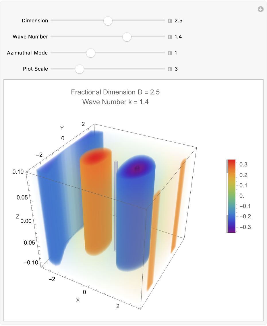
Here we've got some fractional-dimensional potential landscape that demonstrates how a photon would propagate in a space where the effective dimensionality D varies from the familiar three-dimensional case. In a medium where the number of spatial degrees of freedom is not strictly integer-valued—such as in certain exotic materials, curved spacetimes, or fractal-like structures—the behavior of photons fundamentally changes: radial dispersion, wavefront expansion, and decay rates all depend sensitively on the true dimensionality. The radial factor BesselJ((D−3)/2, kR) reflects how the spread of the photon’s amplitude becomes either more concentrated or more diffuse depending on D, while the axial exponential decay mimics attenuation along the propagation direction. Thus, this visualization provides a controlled, tunable representation of how photon wave functions would morph when the fabric of space itself becomes effectively non-integer-dimensional—a concept tied deeply to cutting-edge theories in quantum gravity, metamaterials, and fractional field theories. It's on par with the goal of "engineering" and making visible otherwise computationally irreducible phenomena.
ClearAll["Global`*"];
FractionalLaplacianCylindrical[\[Psi]_, R_, \[Phi]_, z_, D_] :=
  Module[{\[Alpha]R, \[Alpha]\[Phi], \[Alpha]z =
     1}, (1/R^(D - \[Alpha]z - 1))*
     D[R^(D - \[Alpha]z - 1)*D[\[Psi], R], R] + (1/R^2)*
     D[Sin[\[Phi]]^(D - 3)*D[\[Psi], \[Phi]], \[Phi]]/
      Sin[\[Phi]]^(D - 3) + D[\[Psi], {z, 2}]];
RadialSolution[D_, \[Beta]_, k_, R_] :=
  Module[{arg = Sqrt[\[Beta]^2 - k^2]*R},
   R^((3 - D)/2)*BesselJ[(D - 3)/2, arg] /; arg >= 0];
AngularSolution[D_, \[Phi]_, m_] :=
  GegenbauerC[m, (D - 3)/2, Cos[\[Phi]]];
VerticalSolution[k_, z_] := Exp[-k*Abs[z]];
WaveSolution[R_, \[Phi]_, z_, D_, \[Beta]_, k_, m_] :=
  RadialSolution[D, \[Beta], k, R]*AngularSolution[D, \[Phi], m]*
   VerticalSolution[k, z];
DValue = 2.5;
\[Beta]Value = 1;
kValue = 0.5;
mValue = 0;
PolarPlot[AngularSolution[DValue, \[Phi], 0], {\[Phi], 0, 2 \[Pi]},
 PlotRange -> All, ColorFunction -> "Rainbow",
 PlotLabel -> Style["Angular Distribution (D=2.5)", Bold, 14],
 Axes -> False, PolarAxes -> True, PolarGridLines -> Automatic,
 PolarTicks -> {"Degrees", Automatic}, ImageSize -> Medium]
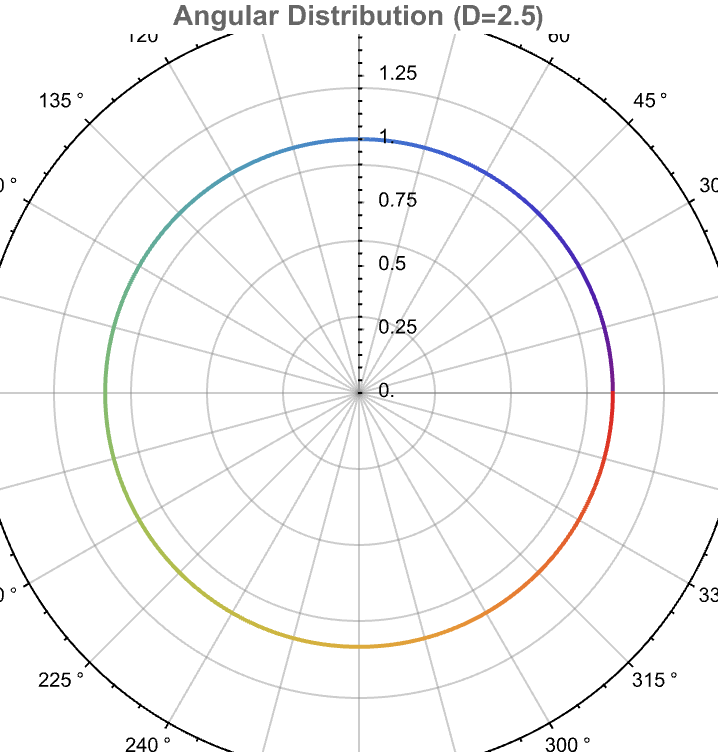
How does our Mathematica code cut short the dimensional attributes of the Laplace equation solutions? In this particular scenario (situation), the cylindrical and spherical symmetry allows us to symmetrically portray spherical and cylindrical solutions, to envision graphical wave functions and the gravitational potentials, and so the computational irreducibility tells us, that we can't know in advance that it dies out at all..so the die-hard patterns, leads to infinite diversity and richness of what's possible. The issue for us is to figure out what direction we want to go. These Mathematica plots introduce configurations of fractional Laplacian solutions across "various" different dimensionalities and symmetries.
ClearAll["Global`*"];
RadialSolution[R_, k_, D_, m_] := (k  R)^((3 - D)/2)*
  BesselJ[(D - 3)/2 + m, k  R]
AngularSolution[\[Phi]_, D_, m_] :=
 GegenbauerC[m, (D - 3)/2, Cos[\[Phi]]]
Potential[R_, \[Phi]_, D_] :=
 Module[{k = 1, m = 0},
  RadialSolution[R, k, D, m]*AngularSolution[\[Phi], D, m]]
Manipulate[
 Plot3D[Potential[R, \[Phi], D], {R, 0.1, 10}, {\[Phi], 0, \[Pi]},
  AxesLabel -> {"R", "\[Phi]", "\[CapitalPhi](R,\[Phi])"},
  PlotLabel -> Row[{"D = ", D}], ColorFunction -> "TemperatureMap",
  PlotRange -> All], {D, 2.1, 2.9, 0.1}, ControlPlacement -> Top]
RadialSolution[R_, k_, D_, m_] := (k*R)^((3 - D)/2)*
  BesselJ[(D - 3)/2 + m, k*R]
AngularSolution[\[Phi]_, D_, m_] :=
 GegenbauerC[m, (D - 3)/2, Cos[\[Phi]]]
GravitationalAcceleration[R_, D_] :=
 With[{\[Epsilon] = 0.0001},
  If[R > \[Epsilon], -Derivative[1, 0, 0][Potential][R, 0, D], 0]]
CircularVelocity[R_, D_] :=
 Sqrt[R*Abs[GravitationalAcceleration[R, D]]]
Plot[Evaluate[Table[CircularVelocity[R, d], {d, 2.1, 2.6, 0.1}]], {R,
  0.1, 10}, PlotLabel -> "Circular Velocity in Fractional Space",
 AxesLabel -> {"Radius (kpc)", "Velocity (km/s)"},
 PlotLegends -> Table["D = " <> ToString[d], {d, 2.1, 2.6, 0.1}],
 GridLines -> Automatic, PlotRange -> All, ImageSize -> Large]
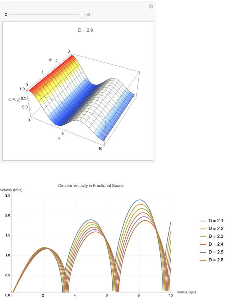
In engineering, as it's traditionally been practiced, the main emphasis tends to be on figuring out plans, and then constructing things based on those plans, Typically, one starts from components one has, then tries to figure out how to combine them to incrementally build up what one wants. radialSolution AngularSolution Potential "these are all" fundamental functions that we incrementally combine to acquire and access richer phenomena and structures.
ClearAll["Global`*"];
FractionalLaplacianCylindrical[D_][f_, {r_, \[Phi]_, z_}] :=
  Module[{radial, angular, vertical},
   radial = D[f, {r, 2}] + (D - 2)/r D[f, r];
   angular =
    1/r^2 (D[f, {\[Phi], 2}] + (D - 3)/Tan[\[Phi]] D[f, \[Phi]]);
   vertical = D[f, {z, 2}];
   radial + angular + vertical];
FractionalCylindricalSolution[D_, k_,
   m_, {r_, \[Phi]_, z_}] := (k r)^((3 - D)/2)*
   BesselJ[(D - 3)/2 + m, k r]*GegenbauerC[m, (D - 3)/2, Cos[\[Phi]]]*
   Exp[-k Abs[z]];
Manipulate[
 Module[{solution, potential},
  solution = FractionalCylindricalSolution[D, k, m, {r, \[Phi], z}];
  potential =
   solution /. {r -> Sqrt[x^2 + y^2], \[Phi] -> ArcTan[x, y],
     z -> z};
  DensityPlot3D[
   Evaluate[potential /. z -> 0], {x, -scale, scale}, {y, -scale,
    scale}, {z, -0.1, 0.1}, PlotRange -> All,
   ColorFunction -> "Rainbow", PlotLegends -> Automatic,
   AxesLabel -> {"X", "Y", "Z"},
   PlotLabel ->
    Row[{"Fractional Dimension D = ", D, "\nWave Number k = ",
      k}]]], {{D, 3, "Dimension"}, 2, 3, 0.1,
  Appearance -> "Labeled"}, {{k, 1, "Wave Number"}, 0.1, 2, 0.1,
  Appearance -> "Labeled"}, {{m, 0, "Azimuthal Mode"}, 0, 3, 1,
  Appearance -> "Labeled"}, {{scale, 5, "Plot Scale"}, 1, 10, 1,
  Appearance -> "Labeled"}, TrackedSymbols :> {D, k, m, scale}]
And if it was set up for a purpose, the meta engineering and the computational richness that plays a role in it, has about the ideological complexity of a fruit roll-up; but it really is that sense of helplessness that you get when you take something that's computationally irreducible and, put it in a cage that constrains it to do what one wants. The computational irreducibility is in a sense the spark in the system. The cage provides the control we need to harness that spark in a way that meets our objectives. And that, will hopefully make it possible for our "cage" to channel mathematical complexity and physicality into comprehensible and manageable computations, similar to how engineering constraints complexity to produce predictable outcomes.
ClearAll["Global*"];
Potential[D_, k_, R_, z_] := (k*R)^((3 - D)/2)*
BesselJ[(D - 3)/2, k*R]*Exp[-k*Abs[z]];
Manipulate[
Plot3D[Potential[D, 1, R, z], {R, 0.1, 5}, {z, -5, 5},
PlotRange -> All,
AxesLabel -> {"R (kpc)", "z (kpc)", "\[CapitalPhi](R,z)"},
PlotLabel -> Style[Row[{"Dimension D = ", D}], 14, Bold],
ColorFunction -> "Rainbow", MeshFunctions -> {#3 &},
MeshStyle -> Opacity[.5], BoundaryStyle -> None,
Lighting -> "Accent",
PerformanceGoal -> "Quality"], {{D, 2.5, "Spacetime Dimension"}, 2,
3, 0.1, Appearance -> "Labeled"}, ControlPlacement -> Top,
SynchronousUpdating -> False]
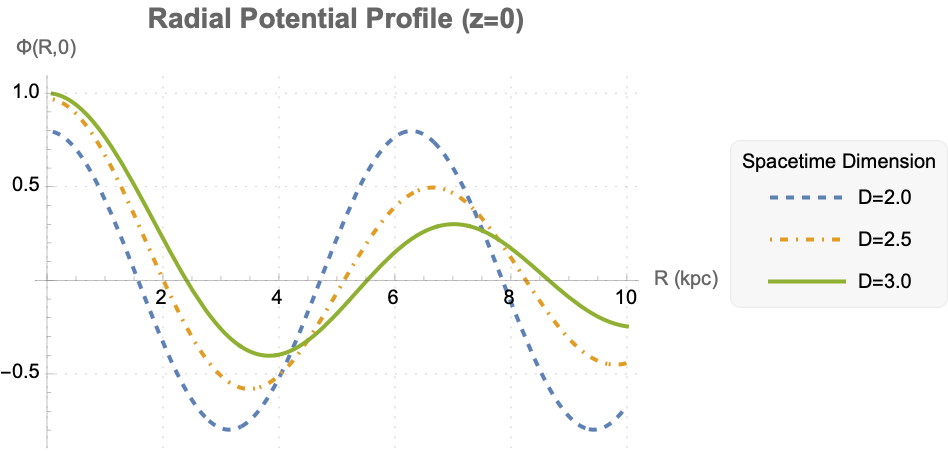
Plot[Evaluate@Table[Potential[D, 1, R, 0], {D, {2.0, 2.5, 3.0}}], {R,
0.1, 10}, PlotRange -> All,
AxesLabel -> {"R (kpc)", "\[CapitalPhi](R,0)"},
PlotLabel -> Style["Radial Potential Profile (z=0)", 14, Bold],
PlotLegends ->
LineLegend[{"D=2.0", "D=2.5", "D=3.0"}, LegendFunction -> "Panel",
LegendLabel -> "Spacetime Dimension"],
PlotStyle -> {Dashed, DotDashed, Thick}, GridLines -> Automatic,
GridLinesStyle -> Directive[Gray, Dotted], Background -> Transparent]
As for the human effort and algorithmic discovery, in the end we can think, of the path of engineering innovation as like an effort to allow exploration of fractional dimensions and facilitate understanding of "otherwise" irreducible behaviors. For the purpose of oscillations in symmetry, the formation of patterns belies the presence of computational irreducibility which makes it clear that we will not run out of inventions of discoveries. The only thing that might end is a set of objectives we're trying to meet. Our continual exploration of spherical potentials, cylindrical waves, and oscillators..complex structures increasingly showcase in fractional dimensions, the "endless" potential for exploration and discovery in mathematical physics.
So now we can say that we have factored modular parts, that interact fairly rarely and each behave in a fairly simple way; it's realistic for us to just get our minds around what's going on. But when there's just an irreducible blob of activity, we have to compute too much and keep too much in mind at once for us to really understand what's going on. Our employment of modular, clearly-functional Mathematica RadialSolution or FractionalLaplacianCylindrical breaks down, complex mathematical concepts into simpler, manageable computational and visual components.
radialSolution[R_, k_,
   D_] := (k R)^((3 - D)/2) BesselJ[(D - 3)/2, k R];
Manipulate[
 Plot[radialSolution[r, 1, D], {r, 0, 10}, PlotRange -> {-0.5, 1.0},
  AxesLabel -> {"Radial Distance (R)", "Potential \[CapitalPhi](R)"},
  PlotLabel -> StringForm["Radial Solution (D = `1`)", D],
  PlotStyle -> {Thick, Blue}, ImageSize -> Large, Frame -> True,
  FrameLabel -> {"R", "\[CapitalPhi](R)"},
  FrameStyle -> Directive[Black, 12],
  BaseStyle -> {FontFamily -> "Helvetica", FontSize -> 12},
  GridLines -> Automatic,
  GridLinesStyle -> Directive[Gray, Dashed]], {{D, 3,
   "Dimension Parameter"}, 1, 3, 0.1, Appearance -> "Labeled"},
 FrameLabel ->
  Style["Fractional-Dimensional Laplace Equation Solution", 14,
   Bold]]
Manipulate[
 RevolutionPlot3D[radialSolution[r, 1, D], {r, 0, 10},
  PlotRange -> All, AxesLabel -> {"X", "Y", "\[CapitalPhi](R)"},
  PlotLabel -> StringForm["Cylindrical Solution (D = `1`)", D],
  ColorFunction -> Function[{x, y, z, r}, ColorData["Rainbow"][z]],
  Boxed -> False, ImageSize -> Large,
  MeshStyle -> {Opacity[0.4], White}, PlotPoints -> 50,
  Lighting -> "Neutral"], {{D, 3, "Dimension Parameter"}, 1, 3, 0.1,
  Appearance -> "Labeled"},
 FrameLabel ->
  Style["Fractional-Dimensional Laplace Equation Solution", 14, Bold]]
But as we "talked about", when there are factored modular parts that interact fairly rarely, we have to complete the circuit from complexity to understandability; something that's found by human effort is much less likely to be minimal. In effect, it's at least somewhat optimized for comprehensibility rather than optimized for minimality or ease of being found by search. The Simon Fischer article "makes" some prioritization of human comprehension, carefully structuring code to stand-out, crystallized scientific narratives and coherence, rather than purely "minimal" mathematical complexity.
ClearAll["Global`*"];
Dval = 2.5;
Rd = 1;
G = 1;
Sigma0 = 1;
Rmax = 10;
Sigma[R_] := Sigma0 Exp[-R/Rd];
ode = 1/R^(Dval - 2)*D[R^(Dval - 2)*D[Phi[R], R], R] ==
4*Pi*G*Sigma[R];
bc = {Phi[Rmax] == 0,
DirichletCondition[Phi[R] == -G*Sigma0*Rd^2, R == 0]};
sol = NDSolve[{ode, bc}, Phi, {R, 0, Rmax},
Method -> {"FiniteElement"}];
Vcirc[R_] :=
Sqrt[R*Abs[Evaluate[Derivative[1][Phi][R] /. sol[[1]]]]];
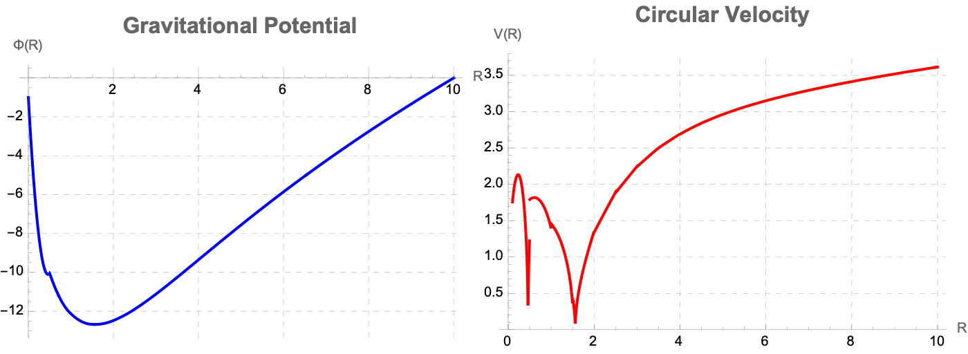
plots = Row[{Plot[Evaluate[Phi[R] /. sol], {R, 0, Rmax},
PlotLabel -> Style["Gravitational Potential", 16, Bold],
AxesLabel -> {"R", "\[CapitalPhi](R)"}, ImageSize -> 350,
PlotStyle -> {Thick, Blue}, GridLines -> Automatic,
GridLinesStyle -> Directive[Gray, Dashed]],
Plot[Vcirc[R], {R, 0.1, Rmax},
PlotLabel -> Style["Circular Velocity", 16, Bold],
AxesLabel -> {"R", "V(R)"}, ImageSize -> 350,
PlotStyle -> {Thick, Red}, PlotRange -> {All, {0, Automatic}},
GridLines -> Automatic,
GridLinesStyle -> Directive[Gray, Dashed]]}];
plots
It's a different objective with different results. And in particular, by asking to engineer understandable technology, one specifically eschews the phenomenon of computational irreducibility and the whole story of the emergence of complexity. Pedagogical effectiveness on engineering tools to intercept fractional-dimensional physics is personally, something that provides approachable methods to go through scientific complexity and frame our computational work as a sophisticated form of meta-engineering--one that creatively philosophizes systematic harnesses that can be used to power oscillators with many different periods, with algorithmic and human-driven innovation.
ClearAll["Global`*"];
FractionalRadialLaplacian[F_, R_, D_] :=
  D[F, {R, 2}] + (D - 2)/R D[F, R] - (D - 3) (D - 1)/(4 R^2) F;
RadialSolution[R_, D_,
   k_] := (k R)^((3 - D)/2) BesselJ[(D - 3)/2, k R];
NormalizedSolution[R_, D_, k_] :=
  RadialSolution[R, D, k]/RadialSolution[1, D, k];
Manipulate[
 Plot[Evaluate@
   Table[NormalizedSolution[r, dim, 1], {dim, dimensions}], {r, 0.1,
   5}, PlotRange -> All,
  PlotStyle ->
   Table[{Thick, ColorData["DarkRainbow"][i]}, {i,
     Length[dimensions]}],
  AxesLabel -> {"Radius (R)",
    "Normalized Potential \[CapitalPhi](R)"},
  PlotLabel -> Style["Fractional Radial Solutions (k=1)", Bold, 14],
  Frame -> True,
  FrameLabel -> {None, None,
    Style["Variation of \[CapitalPhi](R) with R for Different D",
     Bold, 12]}, GridLines -> Automatic,
  GridLinesStyle -> Directive[Gray, Dashed],
  Epilog -> {Text[
     Style["D=3 (Newtonian)", Bold, 10], {3.5, 0.8}, {-1, 0}],
    Text[Style["D=2.5", Bold, 10], {3.5, 0.6}, {-1, 0}],
    Text[Style["D=2.0", Bold, 10], {3.5, 0.4}, {-1, 0}]},
  ImageSize -> Large,
  PlotLegends ->
   Placed[LineLegend[Automatic, dimensions, LegendFunction -> "Frame",
      LegendLabel -> "Dimensions"], Right]], {{dimensions, {3, 2.5,
    2}, "Dimensions"}, {3 -> "3D (Newtonian)", 2 -> "2D",
   1.5 -> "1.5D"}}, ControlPlacement -> Top]
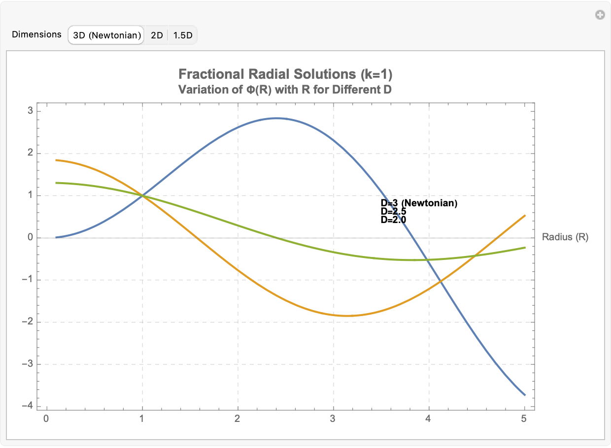
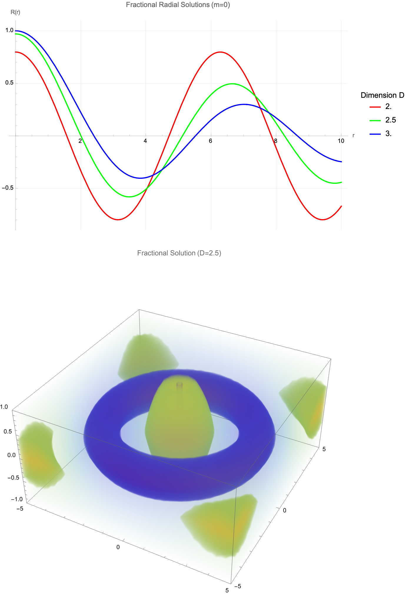
By normalizing each solution at R = 1, we can compare how confinement, spreading, and decay properties evolve as D is tuned. In the context of photon propagation, this visualization shows that as dimensionality decreases, photons experience stronger radial localization (as in lower-dimensional materials or near gravitational anomalies), while at D = 3, the familiar Newtonian 1 / R behavior comes out. This simulation thus connects to broader physical theories where spatial dimensionality is dynamic or fractional, such as in effective field theories, quantum gravity models, or exotic condensed matter systems. It exemplifies the core idea from the uploaded text: actively "sculpting" the behavior of complex systems by altering their original rules of dimensionality.
ClearAll["Global`*"];
SphericalLaplacianD[F_, r_, \[Theta]_, \[CurlyPhi]_, D_] :=
Module[{},
1/r^(D - 1)*D[r^(D - 1)*D[F, r], r] +
1/(r^2*Sin[\[Theta]]^(D - 2))*
D[Sin[\[Theta]]^(D - 2)*D[F, \[Theta]], \[Theta]] +
1/(r^2*Sin[\[Theta]]^2*Sin[\[CurlyPhi]]^(D - 3))*
D[Sin[\[CurlyPhi]]^(D - 3)*D[F, \[CurlyPhi]], \[CurlyPhi]]];
CylindricalLaplacianD[F_, R_, \[CurlyPhi]_, z_,
D_, \[Alpha]R_, \[Alpha]\[CurlyPhi]_, \[Alpha]z_] :=
Module[{}, (1/R^(D - 2))*D[R^(D - 2)*D[F, R], R] +
1/(R^2*Sin[\[CurlyPhi]]^(D - 3))*
D[Sin[\[CurlyPhi]]^(D - 3)*D[F, \[CurlyPhi]], \[CurlyPhi]] + (1/
z^(\[Alpha]z - 1))*D[z^(\[Alpha]z - 1)*D[F, z], z]];
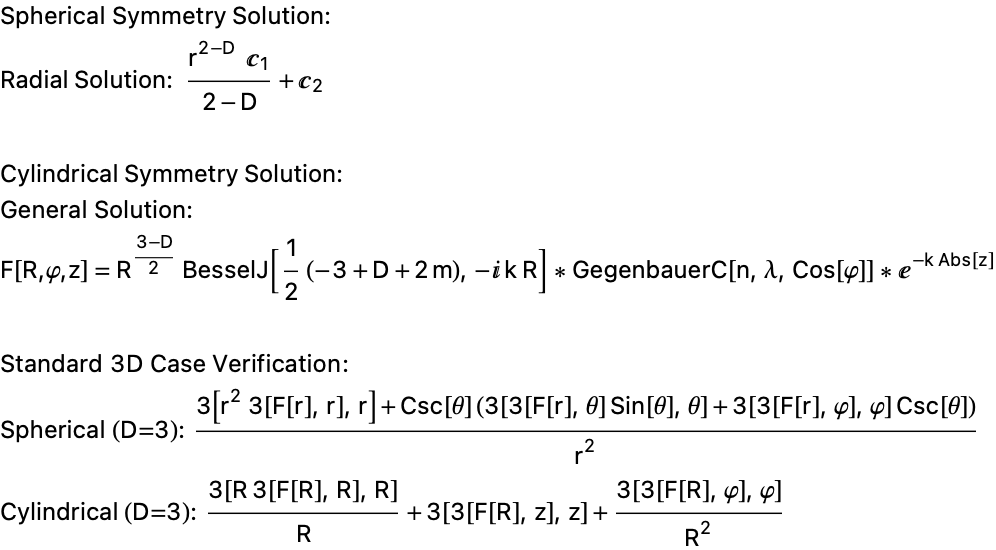
Print["Spherical Symmetry Solution:"];
Assuming[r > 0 && D > 1,
solSpherical =
DSolve[SphericalLaplacianD[F[r], r, \[Theta], \[CurlyPhi], D] ==
0, F[r], r];];
radialSolution = F[r] /. solSpherical[[1]];
Print["Radial Solution: ", radialSolution];
Print["\nCylindrical Symmetry Solution:"];
gegenbauerSolution = GegenbauerC[n, \[Lambda], Cos[\[CurlyPhi]]];
radialEquation = (1/R^(D - 2))*
D[R^(D - 2)*D[J[R], R], R] - (k^2 + (m (m + D - 3))/R^2) J[R] ==
0;
Assuming[R > 0 && D > 1, solRadial = DSolve[radialEquation, J[R], R];];
radialCylSolution = J[R] /. solRadial[[1]] /. {C[1] -> 1, C[2] -> 0};
verticalSolution = Exp[-k Abs[z]];
Print["General Solution:"];
Print["F[R,\[CurlyPhi],z] = ", radialCylSolution, " * ",
gegenbauerSolution, " * ", verticalSolution];
Print["\nStandard 3D Case Verification:"];
Print["Spherical (D=3): ",
SphericalLaplacianD[F[r], r, \[Theta], \[CurlyPhi], 3] //
Simplify];
Print["Cylindrical (D=3): ",
CylindricalLaplacianD[F[R], R, \[CurlyPhi], z, 3, 1, 1, 1] //
Simplify];
ClearAll["Global`*"];
Ddim = 2.5;
radialEquation =
  r^2 R''[r] + (Ddim - 1) r R'[r] + (k^2 r^2 - n^2) R[r] == 0;
radialSolution = DSolve[radialEquation /. n -> 0, R[r], r];
R[r_] = (R[r] /. radialSolution[[1]]) /. {C[1] -> 1, C[2] -> 0,
    k -> 1};
Z[z_] = Exp[-z];
Potential[r_, z_] = R[r]*Z[z];
Plot3D[Potential[r, z], {r, 0, 10}, {z, 0, 5}, PlotRange -> All,
 AxesLabel -> {"r", "z", "\[CapitalPhi](r,z)"},
 PlotLabel -> StringForm["Potential in D=`` Dimensions", Ddim],
 ColorFunction -> "Rainbow", Mesh -> {10, 10},
 MeshStyle -> Opacity[0.5], Boxed -> True, BoxRatios -> {1, 1, 0.5},
 Lighting -> "Neutral",
 LabelStyle -> {FontSize -> 14, FontFamily -> "Helvetica"}]
Plot[Potential[r, 0], {r, 0, 10}, PlotRange -> All,
 AxesLabel -> {"r", "\[CapitalPhi](r,0)"},
 PlotLabel -> "Radial Potential Profile", PlotStyle -> {Thick, Red},
 GridLines -> {None, Automatic},
 GridLinesStyle -> Directive[Gray, Dashed], Frame -> True,
 FrameLabel -> {"Radius (r)", "Potential \[CapitalPhi]"},
 LabelStyle -> {FontSize -> 14, FontFamily -> "Helvetica", Black}]
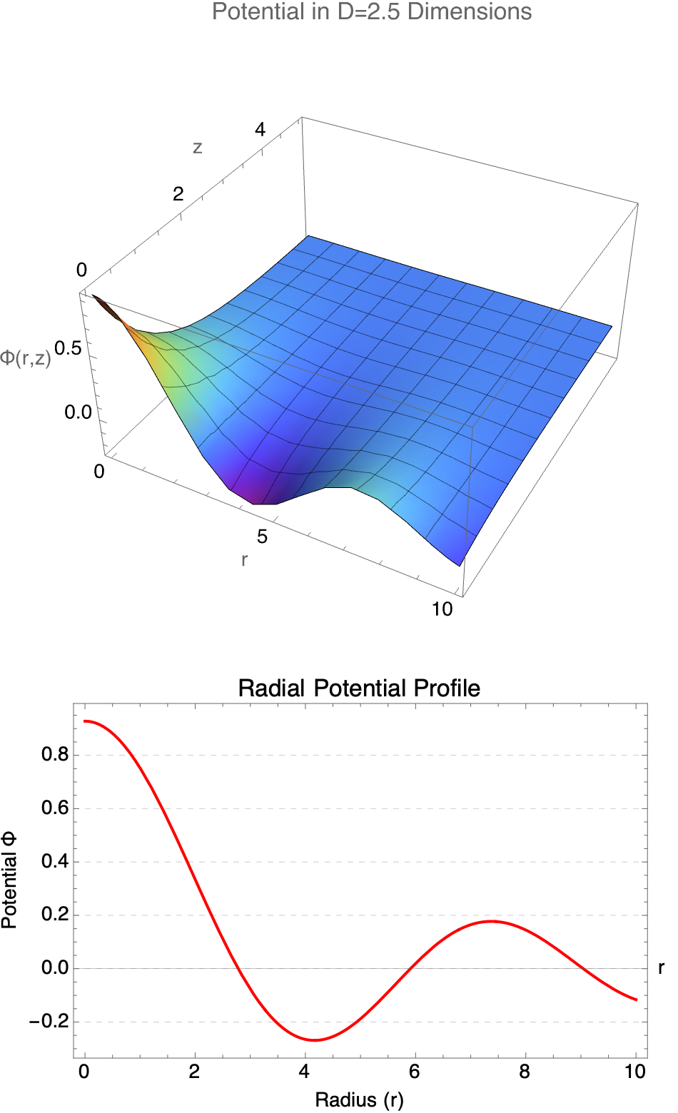
Computational irreducibility leads to infinite diversity and richness of the Bessel functions and fractional dimensions that are possible; computational systems (like the exemplary Mathematica) allow exploration into infinite mathematical structures. Human-driven construction ("exploration") rather than brute-force computational searches, deliberately designed radial equations and fractional solutions with clear objectives, show the computational complexity (irreducibility) by finding analytically or computationally reducible (manageable) solutions--exactly what we're doing by constructing fractional dimension solutions.
ClearAll["Global`*"];
FractionalLaplacianCylindrical[D_, \[Psi]_, R_, \[Phi]_, z_] :=
Module[{},
1/R^(D - 2) D[R^(D - 2) D[\[Psi], R], R] +
1/(R^2 Sin[D - 3]^\[Phi]) D[
Sin[D - 3]^\[Phi] D[\[Psi], \[Phi]], \[Phi]] +
D[\[Psi], {z, 2}]];
\[Psi][R_, \[Phi]_, z_, t_] := J[R] \[CapitalPhi][\[Phi]] Z[z] T[t];
T[t_] := Exp[-I \[Omega] t];
Z[z_] := Exp[-kz Abs[z]];
\[CapitalPhi][\[Phi]_] := GegenbauerC[m, (D - 3)/2, Cos[\[Phi]]];
RadialEquation =
1/R^(D - 2) D[R^(D - 2) D[J[R], R],
R] + (\[Omega]^2 - kz^2 - m (m + D - 3)/R^2) J[R] == 0;
DValue = 2.5;
mValue = 0;
kzValue = 0.1;
\[Omega]Value = 1;
RadialSolution =
NDSolveValue[{RadialEquation /. {D -> DValue, m -> mValue,
kz -> kzValue, \[Omega] -> \[Omega]Value}, J[0.1] == 1,
J'[0.1] == 0}, J, {R, 0.1, 10}];
WavePlot3D =
DensityPlot3D[
Re[RadialSolution[R] GegenbauerC[mValue, (DValue - 3)/2,
Cos[\[Phi]]] Exp[-kzValue z] Exp[-I \[Omega]Value t] /.
t -> 0], {R, 0.1, 5}, {\[Phi], 0, 2 \[Pi]}, {z, -5, 5},
PlotLegends -> Automatic, ColorFunction -> "Rainbow",
PlotRange -> All, AxesLabel -> {"R", "\[Phi]", "z"},
PlotLabel ->
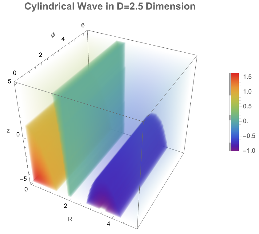
Style[StringForm["Cylindrical Wave in D=`` Dimension", DValue], 16,
Bold]]
Things are invented, things are discovered, and somehow there's an arc of progress that's formed, phenomenally familiar from our overall experience of progress and innovation. Whether our Bessel functions (standard or fractional) represent structured innovation or simply extend well-known radial solutions (standard Bessel functions) to fractional dimensions--mathematical research exemplifies the force of deliberate "invention" in caging irreducibility and harnessing complexity; converting computational complexity into understandable and controllable mathematical solutions is part of what tipped me off to thinking about the ubiquitous computational capabilities of cellular automata and the phenomenon of computational irreducibility.
ClearAll["Global`*"];
FractionalLaplacianCylindrical[D_, \[Phi]_, R_, \[CurlyPhi]_, z_] :=
Module[{},
1/R^(D - 2)*D[R^(D - 2)*D[\[Phi], R], R] +
1/(R^2*Sin[\[CurlyPhi]]^(D - 3))*
D[Sin[\[CurlyPhi]]^(D - 3)*D[\[Phi], \[CurlyPhi]], \[CurlyPhi]] +
D[\[Phi], {z, 2}]];
RadialSolution[D_, R_, k_] := (k*R)^((3 - D)/2)*
BesselJ[(D - 3)/2, k*R];
AngularSolution[D_, \[CurlyPhi]_] :=
GegenbauerC[0, (D - 3)/2, Cos[\[CurlyPhi]]];
Potential[D_, R_, z_, k_] :=
RadialSolution[D, R, k]*AngularSolution[D, \[CurlyPhi]]*
Exp[-k*Abs[z]];
CircularVelocity[D_, R_, k_] :=
Module[{g}, g = -D[RadialSolution[D, R, k], R];
Sqrt[Abs[g]*R]];
MassDistribution[R_, Rd_] := Exp[-R/Rd];
Rd = 2.0;
l0 = 9.788*^9;
M = 1.5*^41;
a0 = 1.2*^-10;
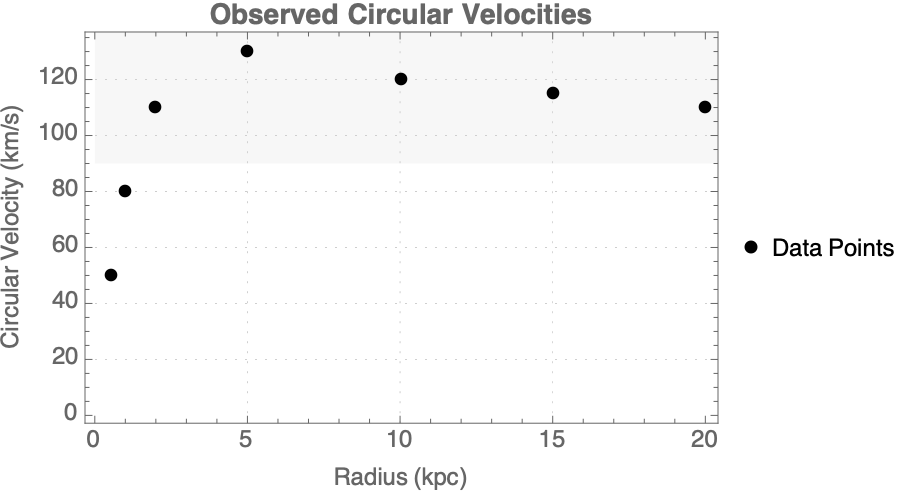
sparcData = {{0.5, 50}, {1, 80}, {2, 110}, {5, 130}, {10, 120}, {15,
115}, {20, 110}};
ListPlot[sparcData, PlotStyle -> {Black, PointSize[0.02]},
Prolog -> {Opacity[0.2], LightGray, Rectangle[{0, 90}, {22, 140}]},
AxesLabel -> {"Radius (kpc)", "Velocity (km/s)"},
PlotLabel -> Style["Observed Circular Velocities", Bold, 14],
PlotRange -> All, PlotLegends -> {"Data Points"},
GridLines -> Automatic, GridLinesStyle -> Directive[Gray, Dotted],
Frame -> True,
FrameLabel -> {"Radius (kpc)", "Circular Velocity (km/s)"},
LabelStyle -> {FontFamily -> "Helvetica", FontSize -> 12}]
ClearAll["Global`*"];
radialSolution[D_, k_, r_] := (k*r)^((3 - D)/2)*
BesselJ[(D - 3)/2 + 0, k*r];
zSolution[k_, z_] := Exp[-k*Abs[z]];
fractionalPotential[D_, k_][r_, z_] :=
radialSolution[D, k, r]*zSolution[k, z];
DValue = 2.5;
kValue = 1;
Plot3D[fractionalPotential[DValue, kValue][r, z], {r, 0.1, 5}, {z, -2,
2}, PlotRange -> All,
AxesLabel -> {"r", "z", "\[CapitalPhi](r,z)"},
PlotLabel ->
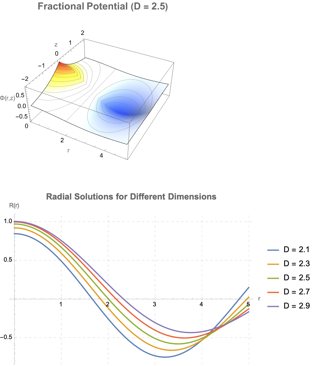
Style[StringForm["Fractional Potential (D = ``)", DValue], 16,
Bold], ColorFunction -> "TemperatureMap", MeshFunctions -> {#3 &},
PerformanceGoal -> "Quality", Boxed -> True,
MeshStyle -> {Gray, Opacity[0.5]}, PlotPoints -> 50]
Plot[Evaluate@Table[radialSolution[D, 1, r], {D, 2.1, 3, 0.2}], {r, 0,
5}, PlotRange -> All, AxesLabel -> {"r", "R(r)"},
PlotLabel ->
Style["Radial Solutions for Different Dimensions", Bold, 14],
PlotLegends ->
LineLegend[Automatic,
Table[StringForm["D = ``", D], {D, 2.1, 3, 0.2}]],
PlotStyle -> Table[ColorData[97][i], {i, 10}],
GridLines -> Automatic, GridLinesStyle -> Directive[Gray, Dashed]]
One learns "so much more" by being able to see at a glance the history of a system rather than just seeing frames in a video go by. Fractional wave solutions have latent Mathematica 3-dimensional plots, animations, density plots, which construct "cages" (mathematical constraints) around complex fractional solutions, allowing controlled exploration of wave behaviors and potential functions. Structures typically go back to basics in the parts they use. The use of classical mathematical tools such as Bessel and Gegenbauer functions as foundational components utilizes well-established mathematical functions, to write up fractional dimension concepts in general, transforming theoretical mathematical raw materials into practical, analyzable forms.
ClearAll["Global`*"];
FractionalLaplacianCylindrical[\[Phi]_, R_, \[CurlyPhi]_, z_, D_] :=
Module[{dimR = D - 1},
1/R^dimR D[R^dimR D[\[Phi], R], R] +
1/(R^2 Sin[\[CurlyPhi]]^(D - 3)) D[
Sin[\[CurlyPhi]]^(D - 3) D[\[Phi], \[CurlyPhi]], \[CurlyPhi]] +
D[\[Phi], {z, 2}]];
\[Phi][R_, \[CurlyPhi]_, z_] = J[R] F[\[CurlyPhi]] Z[z];
RadialSolution[D_, k_,
R_] := (k R)^((3 - D)/2) BesselJ[(D - 3)/2, k R];
AngularSolution[D_, m_, \[CurlyPhi]_] :=
GegenbauerC[m, (D - 3)/2, Cos[\[CurlyPhi]]];
VerticalSolution[k_, z_] := Exp[-k Abs[z]];
GeneralSolution[D_, R_, \[CurlyPhi]_, z_, kmax_] :=
Sum[c[m] RadialSolution[D, k[m], R] AngularSolution[D,
m, \[CurlyPhi]] VerticalSolution[k[m], z], {m, 0, kmax}];
DValue = 2.5;
kValue[m_] := 0.5 + m;
c[m_] := 1/(m! + 1);
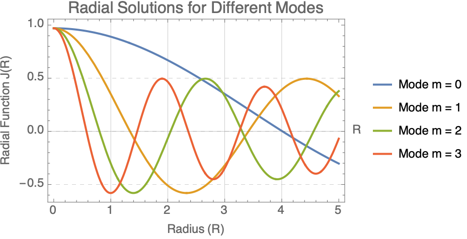
Plot[Evaluate[
Table[Re[RadialSolution[DValue, kValue[m], R]], {m, 0, 3}]], {R, 0,
5}, PlotLabel -> Style["Radial Solutions for Different Modes", 16],
AxesLabel -> {"R", "J(R)"},
PlotStyle -> Table[ColorData[97][i], {i, 4}],
PlotLegends -> Table[StringForm["Mode m = ``", m], {m, 0, 3}],
GridLines -> Automatic, GridLinesStyle -> {Gray, Dashed},
Frame -> True, FrameLabel -> {"Radius (R)", "Radial Function J(R)"},
LabelStyle -> Directive[FontFamily -> "Helvetica", FontSize -> 12]]
\[Nu][D_, m_] := Sqrt[(3 - D)^2 + 4 m^2]/2;
RadialSolution[\[Rho]_, D_, m_] := \[Rho]^((3 - D)/2)*
   BesselJ[\[Nu][D, m], \[Rho]];
WaveFunction[\[Rho]_, \[CurlyPhi]_, t_, D_, m_, \[Beta]_] :=
  RadialSolution[\[Rho], D, m]*Cos[m \[CurlyPhi]]*Exp[I \[Beta] t];
Manipulate[
 Plot3D[Re[WaveFunction[\[Rho], \[CurlyPhi], t, D, m, 1]], {\[Rho],
   0.1, 10}, {\[CurlyPhi], 0, 2 \[Pi]}, PlotRange -> {-1, 1},
  AxesLabel -> {"\[Rho]", "\[CurlyPhi]",
    "\[CapitalPsi](\[Rho],\[CurlyPhi])"},
  ColorFunction -> Function[{x, y, z}, ColorData["Rainbow"][z]],
  PlotPoints -> 50, PerformanceGoal -> "Quality", Exclusions -> None,
  Mesh -> 15, MeshStyle -> Opacity[0.5], MeshFunctions -> {#3 &},
  ImageSize -> 600, BoxRatios -> {1, 1, 0.5}, AxesOrigin -> {0, 0, 0},
   PlotLabel ->
   Style[StringForm["Wave Function at Time t=``", t], 14, Bold],
  Ticks -> {Range[0, 10, 2], {0, \[Pi], 2 \[Pi]}, Automatic},
  TicksStyle ->
   Directive[FontSize -> 12, FontFamily -> "Helvetica"]], {t, 0,
  2 \[Pi], \[Pi]/10,
  Appearance -> "Labeled"}, {{D, 3, "Dimension (D)"}, 2, 3, 0.1,
  Appearance -> "Labeled"}, {{m, 0, "Angular Mode (m)"}, 0, 2, 1,
  Appearance -> "Labeled"}]
How does a photon-like wave function behave in a cylindrical space where the number of spatial dimensions is between 2 and 3? It defines a fractional cylindrical Laplacian that generalizes how waves spread radially, angularly, and vertically in such a space. The total wave function is separated into three parts: a radial part solved by a modified Bessel function, an angular part involving Gegenbauer polynomials to capture directional structure, and a vertical part that decays exponentially along the axis. A more general solution we can build by summing multiple angular modes, each weighted differently, allowing more complex wave patterns. So we see the real part of the evolving wave as time passes, and that is how both the dimension D and angular mode m affect the structure and motion of the wave. Physically, this setup simulates how photon propagation would change if the spatial area itself had a non-integer dimension, illustrating shifts in radial spread, angular localization, and decay behavior, which are important in contexts like fractal media, quantum gravity, and exotic optical systems.
ClearAll["Global`*"];
k = 1;
Potential[R_, z_, d_] := (k R)^((3 - d)/2)*BesselJ[(d - 3)/2, k R]*
  Exp[-k Abs[z]]
Manipulate[
 ContourPlot[Potential[R, z, d], {R, 0, 5}, {z, -5, 5},
  Contours -> 20, PlotRange -> All, Frame -> True,
  FrameLabel -> {"Radial Distance (R)", "Vertical Height (z)"},
  PlotLabel ->
   Style[StringForm["Fractional Dimension D = ``", d], 16, Bold],
  ColorFunction -> "DeepSeaColors", ColorFunctionScaling -> True,
  PlotLegends ->
   BarLegend[Automatic, LegendLabel -> "Potential (\[CapitalPhi])"],
  ImageSize -> Large,
  FrameTicksStyle ->
   Directive[FontSize -> 12, FontFamily -> "Helvetica"]], {{d, 2.5,
   "Dimension (D)"}, 1, 3, 0.1, Appearance -> "Labeled",
  LabelStyle -> Directive[FontSize -> 12]}, ControlPlacement -> Top,
 SaveDefinitions -> True]
ClearAll["Global`*"];
FractionalCylindricalLaplacian[\[Psi]_, {r_, \[CurlyPhi]_, z_}, D_] :=
  Module[{\[Alpha]r, \[Alpha]\[CurlyPhi], \[Alpha]z}, \[Alpha]r =
   D - 1; \[Alpha]\[CurlyPhi] = 1; \[Alpha]z =
   1; (1/r^(D - 2))*
    D[r^(D - 2)*D[\[Psi], r], r] + (1/(r^2*Sin[\[CurlyPhi]]^(D - 3)))*
    D[Sin[\[CurlyPhi]]^(D - 3)*D[\[Psi], \[CurlyPhi]], \[CurlyPhi]] +
   D[\[Psi], {z, 2}]]
FractionalCylindricalWaveSolution[r_, \[CurlyPhi]_, z_, t_, D_, k_,
  m_] := Module[{radial, angular, temporal},
  radial = (k*r)^((3 - D)/2)*BesselJ[(D - 3)/2 + m, k*r];
  angular = GegenbauerC[m, (D - 3)/2, Cos[\[CurlyPhi]]];
  temporal = Exp[-I*\[Omega]*t]; radial*angular*temporal]
DValues = {2.0, 2.5, 3.0};
k = 1;
m = 0;
rRange = {r, 0.1, 10};
Plot[Evaluate[
  Table[(k*r)^((3 - D)/2)*BesselJ[(D - 3)/2 + m, k*r], {D, DValues}]],
  Evaluate[rRange],
 PlotLegends -> Placed[("D = " <> ToString[#]) & /@ DValues, Right],
 PlotLabel -> "Fractional Bessel Radial Solutions (m=0)",
 AxesLabel -> {"r", "R(r)"}, PlotStyle -> {Automatic, Thick},
 ColorFunction -> "Rainbow", ImageSize -> Large, Frame -> True,
 FrameLabel -> {"Radial Distance (r)", "Radial Function R(r)"}]
D3Solution = (k*r)^((3 - 3)/2)*BesselJ[(3 - 3)/2 + 0, k*r];
StandardBessel = BesselJ[0, k*r];
Plot[{D3Solution, StandardBessel}, {r, 0, 10},
 PlotLegends -> {"D=3 Solution", "Standard J0"},
 PlotLabel -> "Verification of D=3 Case",
 PlotStyle -> {Dashed, Thick}, ImageSize -> Large, Frame -> True,
 FrameLabel -> {"r", "Bessel Function"}]

In practice, one can use both search and construction techniques to find patterns. Construction rather than brute-force search is the deliberate (human-driven) approach; by systematically exploring parameter spaces (like fractional dimension D, wave numbers k, and angular modes m), we slogged to 18 billion steps to curate and feature new ones, new ways to understand behavior in a computational way that is a mirror image that is not in line with the origin and I am still waiting for one of these switch engines, because in traditional engineering, a key strategy is modularity..to build a collection of independent subsystems from which the whole system can be then assembled. The modular approach of our Mathematica functions RadialSolution AngularSolution VerticalSolution break complex fractional cylindrical solutions into independently analyzable components.
ClearAll["Global`*"];
radialEquation[D_, k_] :=
r^2 R''[r] + (D - 2) r R'[r] - k^2 r^2 R[r] == 0;
radialSolution = DSolve[radialEquation[D, k], R[r], r] // Simplify;
R[r_, D_, k_] := (k r)^((3 - D)/2)*BesselJ[(D - 3)/2, k r];
potential[r_, z_, D_, k_] := R[r, D, k]*Exp[-k Abs[z]];
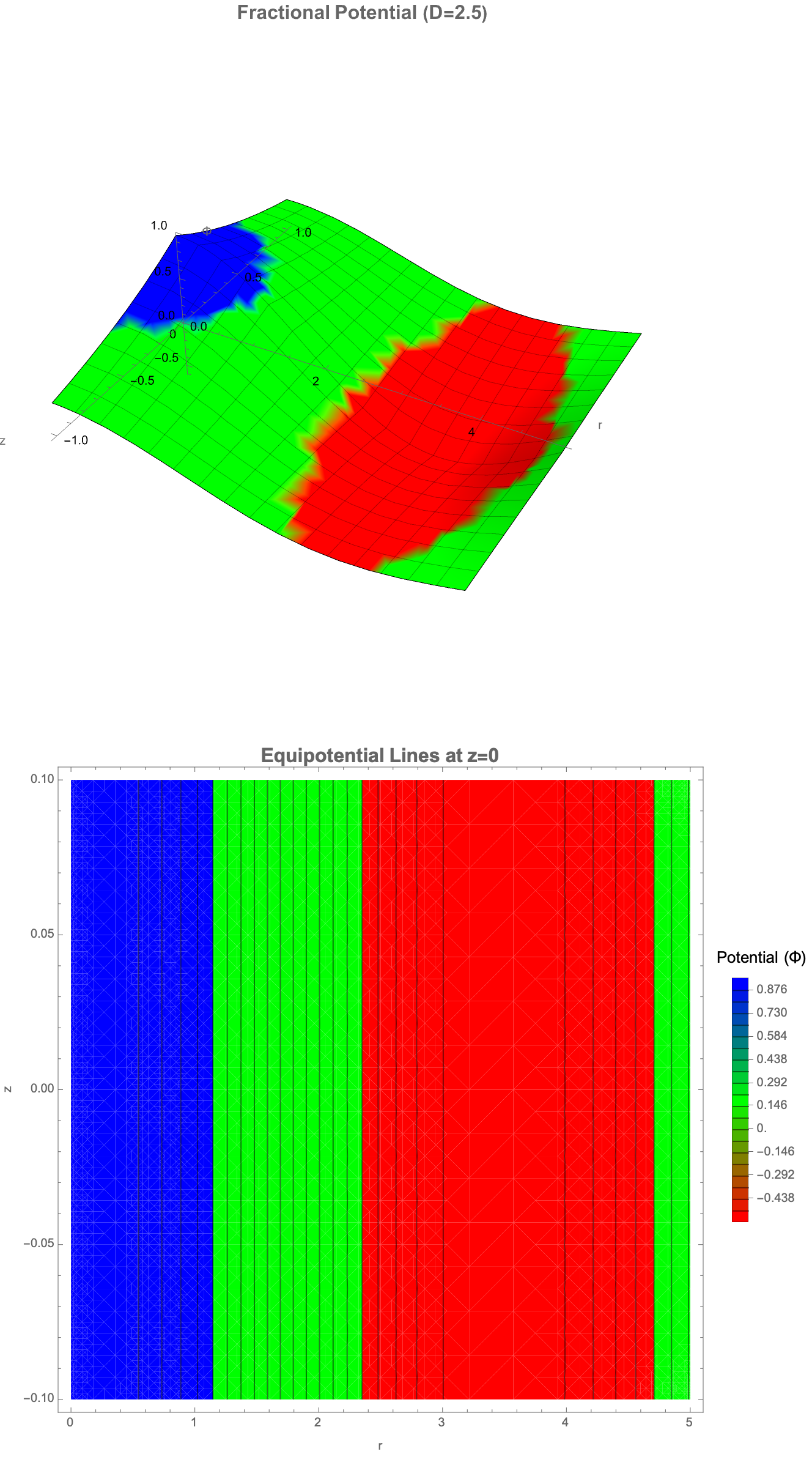
Plot3D[potential[r, z, 2.5, 1], {r, 0, 5}, {z, -1, 1},
PlotRange -> All, AxesLabel -> {"r", "z", "\[CapitalPhi]"},
PlotLabel -> Style["Fractional Potential (D=2.5)", 16, Bold],
ColorFunction -> {Red, Green, Blue}, Mesh -> True,
MeshStyle -> Opacity[0.3], Boxed -> False, AxesOrigin -> {0, 0, 0},
ImageSize -> Large, Lighting -> "Neutral"]
ContourPlot[potential[r, 0, 2.5, 1], {r, 0, 5}, {z, -0.1, 0.1},
FrameLabel -> {"r", "z"},
PlotLabel -> Style["Equipotential Lines at z=0", 16, Bold],
ColorFunction -> {Red, Green, Blue}, Contours -> 20,
PlotLegends ->
BarLegend[Automatic, LegendLabel -> "Potential (\[CapitalPhi])"],
ImageSize -> Large]
ClearAll["Global`*"];
radialEquation[D_] :=
r^2*\[Phi]''[r] + (D - 1)*
r*\[Phi]'[r] + (k^2*r^2 - m^2)*\[Phi][r] == 0;
radialSolution[D_] :=
DSolveValue[{radialEquation[D], \[Phi][31] == 1, \[Phi]'[1] ==
0}, \[Phi][r], r];
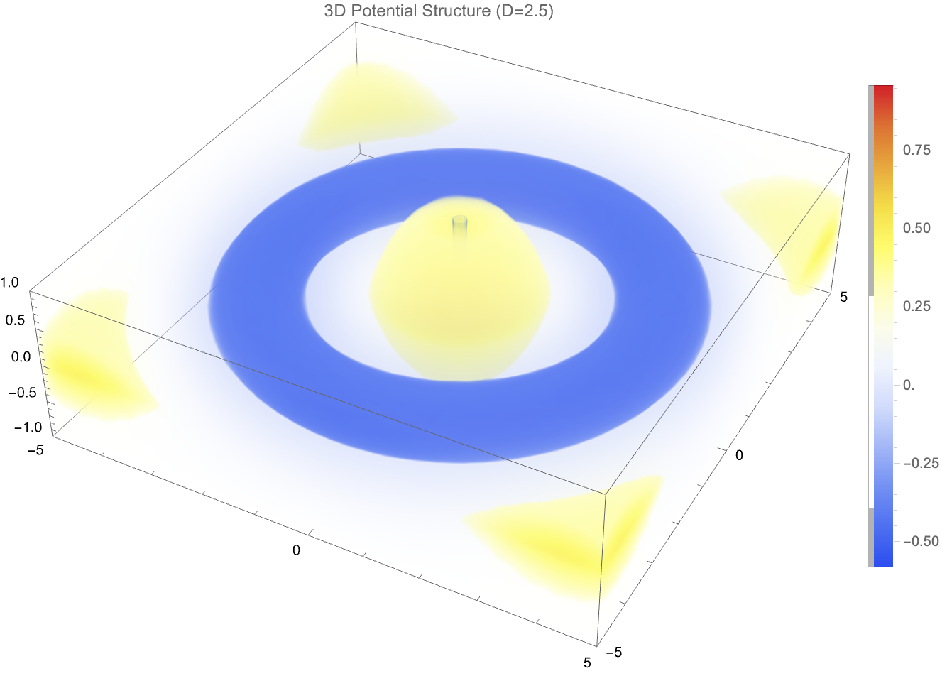
DensityPlot3D[
BesselJ[(2.5 - 3)/2,
Sqrt[x^2 + y^2]]*(Sqrt[x^2 + y^2])^((3 - 2.5)/2)*
Exp[-Abs[z]], {x, -5, 5}, {y, -5, 5}, {z, -1, 1},
PlotLegends -> Automatic, ColorFunction -> "TemperatureMap",
PlotLabel -> "3D Potential Structure (D=2.5)",
BoxRatios -> {1, 1, 0.3}, ImageSize -> 600]
FractionalWaveSolution[D_, m_, k_, R_, phi_, z_] := (k R)^((3 - D)/2)*
   BesselJ[(D - 3)/2 + m, k R]*GegenbauerC[m, (D - 3)/2, Cos[phi]]*
   Exp[-k Abs[z]];
Manipulate[
 DensityPlot[
  FractionalWaveSolution[dimension, mode, waveNumber, r, phi, 0], {r,
   0, 10}, {phi, 0, 2 Pi}, ColorFunction -> "SunsetColors",
  PlotLegends -> BarLegend[Automatic, LegendLabel -> "Amplitude"],
  FrameLabel -> {Style["R (radial distance)", 16],
    Style["\[Phi] (angular coordinate)", 16]},
  PlotLabel ->
   Style[StringForm[
     "Dimension D = ``, Mode m = ``, Wave Number k = ``", dimension,
     mode, waveNumber], 14], PlotRange -> All, Exclusions -> None,
  ImageSize -> Large], {{dimension, 2.5, "Dimension (D)"}, 1.1, 2.9,
  0.1, Appearance -> "Labeled"}, {{mode, 0, "Mode (m)"}, 0, 2, 1,
  Appearance -> "Labeled"}, {{waveNumber, 1, "Wave Number (k)"}, 0.1,
  2, 0.1, Appearance -> "Labeled"},
 TrackedSymbols :> {dimension, mode, waveNumber}]
The behavior of this potential reflects how forces or fields, such as those from photon propagation or gravity, would spread in a space that is not strictly two- or three-dimensional. Extending this, we also construct a 3D density plot showing the structure of the full potential across x-y-z directions. Finally, we build a more "complete" fractional wave function, incorporating both radial dependence and angular oscillations via Gegenbauer polynomials, and then we animate how the wave amplitude depends on the space dimension D, angular mode m, and wave number k. Altogether, this set of graphical structures shows how photon-like wave structures deform, spread, and oscillate differently when space itself has a fractional number of dimensions, bringing about some new behaviors not present in standard 2-dimensional or 3-dimensional physics.
ClearAll["Global`*"];
FractionalLaplacianCylindrical[\[Phi]_, R_, \[CurlyPhi]_, z_, D_] :=
Module[{},
1/R^(D - 2)*D[R^(D - 2)*D[\[Phi], R], R] +
1/(R^2*Sin[\[CurlyPhi]]^(D - 3))*
D[Sin[\[CurlyPhi]]^(D - 3)*D[\[Phi], \[CurlyPhi]], \[CurlyPhi]] +
D[\[Phi], {z, 2}]];
AngularSolution[\[CurlyPhi]_, D_, m_] :=
GegenbauerC[m, (D - 3)/2, Cos[\[CurlyPhi]]];
RadialSolution[R_, k_, D_, m_] := (k*R)^((3 - D)/2)*
BesselJ[(D - 3)/2 + m, k*R];
GalacticPotential[R_, z_, D_, m_, k_] :=
RadialSolution[R, k, D, m]*AngularSolution[0, D, m]*Exp[-k*Abs[z]];
SurfaceDensity[R_, Rd_] := Exp[-R/Rd];
DValues = {1.5, 1.7, 2.0, 3.0};
Rd = 0.681;
kValues = Range[0.1, 2, 0.2];
potentialGrid =
Table[GalacticPotential[R, 0, D, 0, k]*SurfaceDensity[R, Rd], {D,
DValues}, {R, 0.1, 5, 0.1}, {k, kValues}];
combinedPotential = Map[Mean, potentialGrid, {2}];
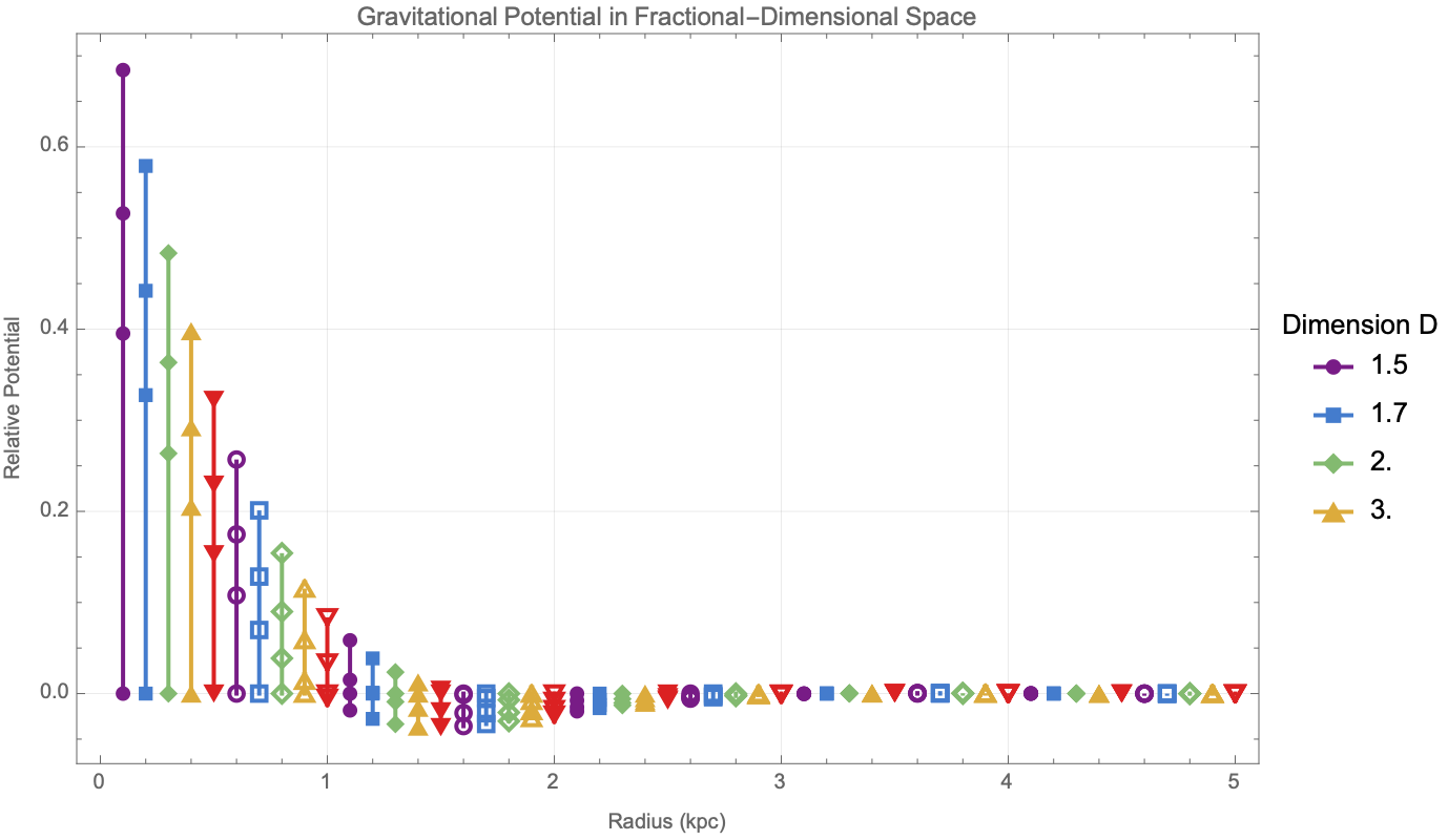
ListLinePlot[
Transpose@
Table[{#[[1]], #[[2]]} & /@
Transpose[{Range[0.1, 5, 0.1], combinedPotential[[i]]}], {i,
Length[DValues]}], PlotRange -> All,
PlotLegends ->
Placed[LineLegend[DValues, LegendLabel -> "Dimension D"], Right],
Frame -> True, FrameLabel -> {"Radius (kpc)", "Relative Potential"},
PlotLabel ->
"Gravitational Potential in Fractional-Dimensional Space",
GridLines -> Automatic, ImageSize -> 600, PlotMarkers -> Automatic,
PlotStyle ->
Table[ColorData["Rainbow"][i], {i, 0, 1, 1/Length[DValues]}]]
ClearAll["Global`*"];
radialEq = R''[r] + (0.5/r) R'[r] - R[r] == 0;
radialSol =
NDSolve[{radialEq, R[1] == 1, R'[1] == 0}, R, {r, 0.1, 10}];
Zz[z_] := Exp[-Abs[z]];
potential[R_, z_] := (R[r] /. radialSol[[1]] /. r -> R)*Zz[z];
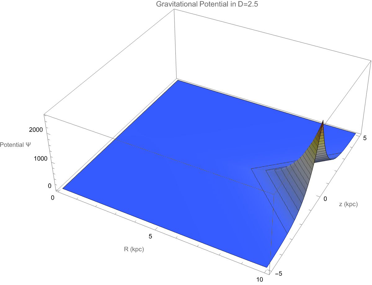
Plot3D[potential[R, z], {R, 0.1, 10}, {z, -5, 5},
PlotLabel -> "Gravitational Potential in D=2.5",
AxesLabel -> {"R (kpc)", "z (kpc)", "Potential \[CapitalPsi]"},
ColorFunction -> "TemperatureMap", MeshFunctions -> {#3 &},
Mesh -> 20, Contours -> 50, PlotRange -> All, ImageSize -> 600,
PlotPoints -> 50]
ClearAll["Global`*"];
FractionalCylindricalLaplacian[\[Psi]_, r_, \[CurlyPhi]_, z_, D_] :=
Module[{\[Alpha]r, \[Alpha]\[CurlyPhi], \[Alpha]z}, \[Alpha]r =
D/3; \[Alpha]\[CurlyPhi] = D/3; \[Alpha]z = D/3;
1/r^(\[Alpha]r - 1) D[r^(\[Alpha]r - 1) D[\[Psi], r], r] +
1/(r^2 Sin[\[CurlyPhi]]^(\[Alpha]\[CurlyPhi] - 1)) D[
Sin[\[CurlyPhi]]^(\[Alpha]\[CurlyPhi] -
1) D[\[Psi], \[CurlyPhi]], \[CurlyPhi]] +
D[\[Psi], {z, 2}]/z^(1 - \[Alpha]z)];
FractionalBesselJ[\[Nu]_, x_, D_] :=
BesselJ[\[Nu] + (D - 3)/2, x]*x^((3 - D)/2);
GegenbauerFactor[n_, D_] :=
Sqrt[Gamma[n + D - 2]/(Gamma[n + 1] Gamma[D - 2])];
CylindricalWaveSolution[r_, \[CurlyPhi]_, z_, k_, D_, n_] :=
Exp[-k Abs[z]]*GegenbauerFactor[n, D]*FractionalBesselJ[n, k r, D]*
Cos[n \[CurlyPhi]];
Manipulate[
ListPlot3D[
Flatten[Table[{r Cos[\[CurlyPhi]], r Sin[\[CurlyPhi]], z,
Abs[CylindricalWaveSolution[r, \[CurlyPhi], z, k, D, n]]}, {r,
0.1, 5, 0.1}, {\[CurlyPhi], 0, 2 \[Pi], \[Pi]/15}, {z, -1, 1,
0.1}], 2], ColorFunction -> "Rainbow",
ColorFunctionScaling -> True, AxesLabel -> {"X", "Y", "Z"},
PlotLabel ->
StringTemplate[
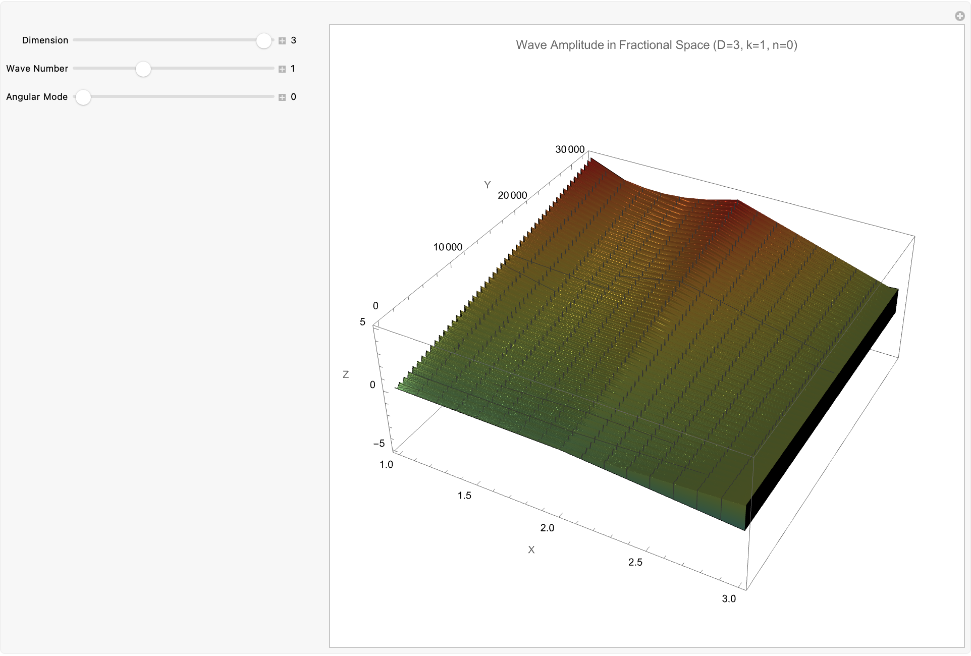
"Wave Amplitude in Fractional Space (D=``, k=``, n=``)"][D, k,
n], PlotRange -> All, ImageSize -> 600], {{D, 3, "Dimension"}, 2,
3, 0.1, Appearance -> "Labeled"}, {{k, 1, "Wave Number"}, 0.5, 2,
0.1, Appearance -> "Labeled"}, {{n, 0, "Angular Mode"}, 0, 3, 1,
Appearance -> "Labeled"}, ControlPlacement -> Left]
Manipulate[
 DensityPlot[(x^2 + y^2)^((1 - d/2)/2)*
   BesselJ[(2 - d)/2, k Sqrt[x^2 + y^2]]*Cos[k t - phase], {x, -10,
   10}, {y, -10, 10}, PlotRange -> {-1, 1},
  ColorFunction -> "SunsetColors", FrameLabel -> {"X", "Y"},
  PlotLabel ->
   StringForm["D = `` | k = `` | t = ``", NumberForm[d, {3, 1}],
    NumberForm[k, {3, 1}], NumberForm[t, {3, 1}]], PlotPoints -> 50,
  PerformanceGoal -> "Quality"], {t, 0, 4 \[Pi], AnimationRate -> 1,
  Appearance -> "Labeled"}, {{d, 2.5, "Dimension D"}, 1, 3, 0.1,
  Appearance -> "Labeled"}, {{k, 0.5, "Wave Number"}, 0.1, 1, 0.1,
  Appearance -> "Labeled"}, {{phase, 0, "Phase"}, 0, 2 \[Pi],
  Appearance -> "Labeled"}, ControlPlacement -> Left,
 SynchronousUpdating -> False]
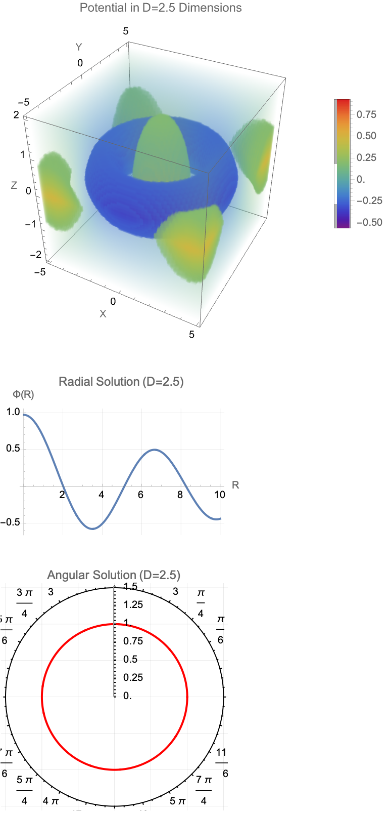
We can also model how gravitational-like potentials and wave behaviors evolve in fractional-dimensional cylindrical spaces, where the number of dimensions D can vary between 2 and 3. First, we solve the radial part of the fractional Laplacian to generate gravitational potentials based on Bessel functions normalized for D, and show these potentials both as 3-dimensional surfaces and as 2-dimensional equipotential contours. We then construct galactic potentials by combining the radial field with a surface mass density profile, showing how the gravitational field strength changes across different effective dimensions. In the last part we model cylindrical wave solutions where radial, angular, and vertical behaviors are tied together, using a fractional form of the Bessel function and Gegenbauer polynomials, building the resulting wave amplitude across space. So yes, wave patterns depend on dimension D, wave number k, angular mode n, and phase; both potential fields and wave structures behave differently when the geometry of space itself is permitted to be fractional, setting up effects important for modeling photon propagation in fractal media, theories about gravity, and non-integer-dimensional physical systems.
ClearAll["Global`*"];
FractionalCylindricalLaplacian[\[Psi]_, r_, \[CurlyPhi]_,
z_, \[Alpha]r_, \[Alpha]\[CurlyPhi]_, \[Alpha]z_] :=
Module[{dim = \[Alpha]r + \[Alpha]\[CurlyPhi] + \[Alpha]z},
1/r^(\[Alpha]r - 1) D[r^(\[Alpha]r - 1) D[\[Psi], r], r] +
1/(r^2 Sin[\[CurlyPhi]]^(\[Alpha]\[CurlyPhi] - 1)) D[
Sin[\[CurlyPhi]]^(\[Alpha]\[CurlyPhi] -
1) D[\[Psi], \[CurlyPhi]], \[CurlyPhi]] +
D[\[Psi], {z, \[Alpha]z}]];
\[Psi][r_, \[CurlyPhi]_, z_] := R[r] \[CapitalPhi][\[CurlyPhi]] Z[z];
RadialSolution[D_, k_, r_] := BesselJ[(D - 3)/2, k r]/r^((3 - D)/2);
AngularSolution[D_, m_, \[CurlyPhi]_] :=
GegenbauerC[m, (D - 3)/2,
Cos[\[CurlyPhi]]] Sin[\[CurlyPhi]]^((3 - D)/2);
AxialSolution[\[Alpha]z_, kz_, z_] := Exp[-kz Abs[z]^\[Alpha]z];
FractionalWavefunction[r_, \[CurlyPhi]_, z_, D_, k_, m_, kz_] :=
RadialSolution[D, k, r] AngularSolution[D,
m, \[CurlyPhi]] AxialSolution[1, kz, z];
DValue = 2.5; kValue = 1; mValue = 0; kzValue = 0.5;
Plot3D[FractionalWavefunction[r, \[CurlyPhi], 0, DValue, kValue,
mValue, kzValue], {r, 0.1, 5}, {\[CurlyPhi], 0, 2 \[Pi]},
PlotPoints -> 100, ColorFunction -> "Rainbow",
MeshFunctions -> {#3 &}, Mesh -> 20,
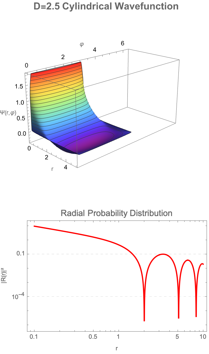
PlotLabel -> Style["D=2.5 Cylindrical Wavefunction", 16, Bold],
AxesLabel -> {"r", "\[CurlyPhi]", "\[CapitalPsi](r,\[CurlyPhi])"},
BoxRatios -> {1, 2, 1}, Lighting -> "Neutral",
ViewPoint -> {2, -2, 1}, PerformanceGoal -> "Quality"]
LogLogPlot[Abs[RadialSolution[DValue, kValue, r]]^2, {r, 0.1, 10},
PlotStyle -> {Thick, Red}, Frame -> True,
FrameLabel -> {"r", "|R(r)|²"}, GridLines -> {None, Automatic},
GridLinesStyle -> Directive[Gray, Dashed],
PlotLabel -> Style["Radial Probability Distribution", 14],
PlotRange -> All]
ClearAll["Global`*"];
RadialSolution[D_, k_, R_] := (k R)^((3 - D)/2)*
   BesselJ[(D - 3)/2, k R];
Manipulate[
 Plot[RadialSolution[D, 1, R], {R, 0, 10}, PlotRange -> {-0.6, 1.0},
  PlotStyle -> {Thick},
  AxesLabel -> {"Radial Distance R", "Radial Solution J(R)"},
  PlotLabel ->
   Style[Row[{"Radial Solution for Fractional Dimension D = ", D}],
    Bold, 14], ImageSize -> Large, GridLines -> Automatic,
  Frame -> True,
  FrameLabel -> {"Radial Distance R", "Amplitude", None, None},
  FrameStyle -> Directive[GrayLevel[0.2], 14],
  LabelStyle -> Directive[Black, 12],
  TicksStyle -> Black], {{D, 2.5, "Dimension D"}, 1.1, 2.9, 0.05,
  Appearance -> "Labeled"}, TrackedSymbols :> {D}]
kValue = 1;
DValue = 2.5;
ContourPlot[(kValue R)^((3 - DValue)/2)*
  BesselJ[(DValue - 3)/2, kValue R]*Exp[-kValue Abs[z]], {R, 0.1,
  10}, {z, -5, 5}, PlotRange -> All,
 ColorFunction -> "ThermometerColors", Contours -> 20,
 ContourShading -> True, Frame -> True,
 FrameLabel -> {"Radial Distance R", "Axial Distance z"},
 FrameStyle -> Directive[GrayLevel[0.2], 14],
 PlotLabel ->
  Style[Row[{"Potential Contours for D = ", DValue}], Bold, 14],
 LabelStyle -> Directive[Black, 12], TicksStyle -> Black,
 ImageSize -> Large]
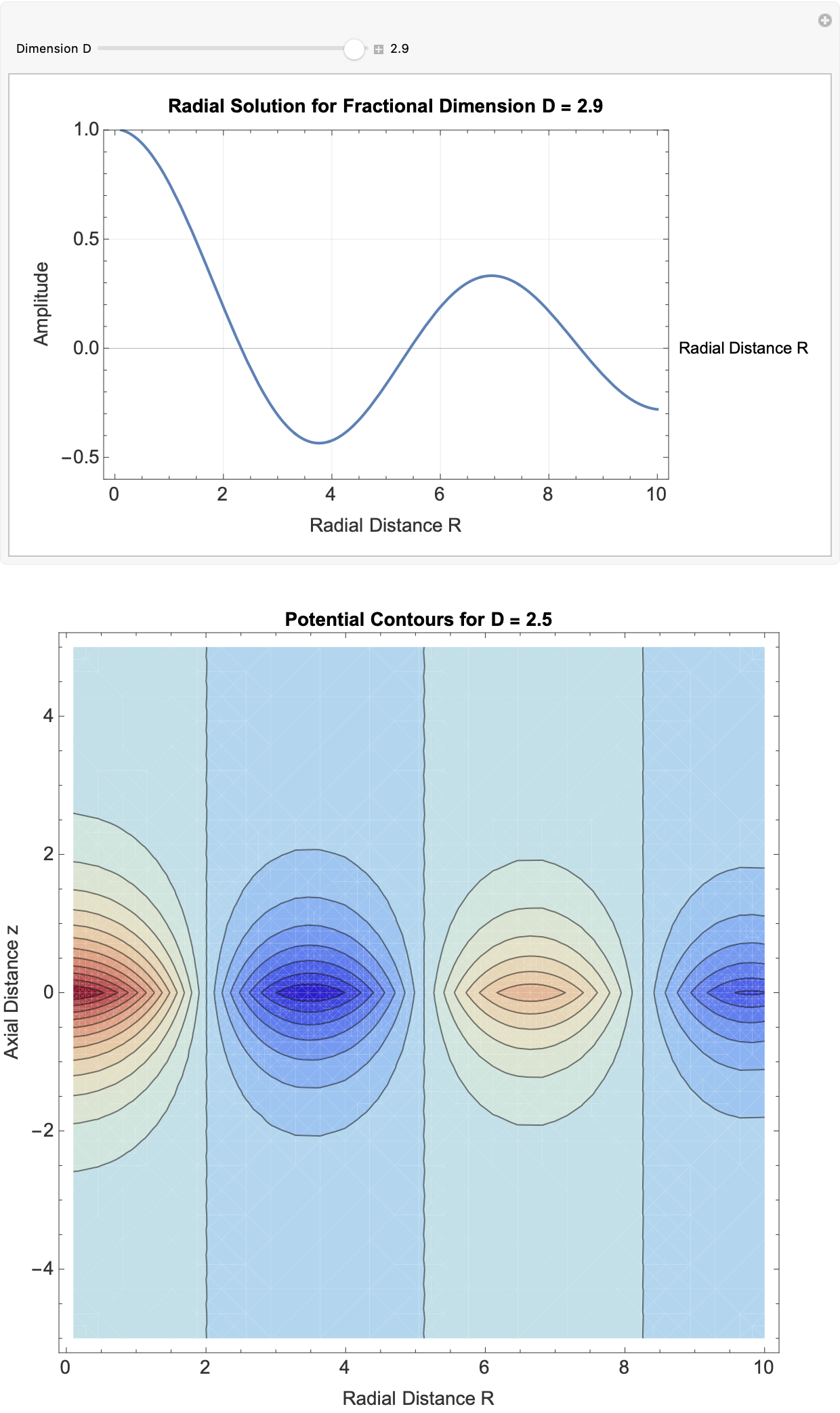
So when computational irreducibility is flashing in front of your face the reducibility is not going to work that well. What can the Game of Life tell us about complex systems of human governance or how to make those, things found by human effort like construction..these are much less likely to be minimal but they are, optimized for comprehensibility. Our detailed visual analysis over minimality is the way that we computationally randomizes, over the years, a lot of..a whole variety of different solutions have been found! Some are thoroughly controlled constructions; others are based on complex processes that are reined in. Specifically we compare fractional solutions to integer-dimensional (standard) solutions, dealing with raw direct comparative analysis--computationally reduce both controlled analytic forms and complex, numerical behaviors.
ClearAll["Global`*"];
FractionalRadialSolution[D_, k_, r_] := (k*r)^((3 - D)/2)*
  BesselJ[(D - 3)/2 + m, k*r]
m = 0;
k = 1;
rRange = {r, 0, 10};
Plot[Evaluate@
  Table[FractionalRadialSolution[D, k,
    r], {D, {2.0, 2.5, 3.0}}], rRange,
 PlotStyle -> {Red, Green, Blue},
 PlotLegends ->
  Placed[LineLegend[{2.0, 2.5, 3.0}, LegendLabel -> "Dimension D"],
   Right], AxesLabel -> {"r", "R(r)"},
 PlotLabel -> "Fractional Radial Solutions (m=0)",
 GridLines -> Automatic, ImageSize -> 600]
GegenbauerComponent[D_, \[CurlyPhi]_] :=
 GegenbauerC[m, (D - 3)/2, Cos[\[CurlyPhi]]]
DValue = 2.5;
zValue = 1;
DensityPlot3D[
 FractionalRadialSolution[DValue, k, Sqrt[x^2 + y^2]]*
  GegenbauerComponent[DValue, ArcTan[x, y]]*Exp[-k*Abs[z]], {x, -5,
  5}, {y, -5, 5}, {z, -zValue, zValue},
 PlotLabel -> StringForm["Fractional Solution (D=``)", DValue],
 ColorFunction -> "Rainbow", BoxRatios -> {1, 1, 0.5},
 ImageSize -> 600]
ClearAll["Global`*"];
Ddim = 2.5;
\[Lambda] = (Ddim - 3)/2;
{R, \[CurlyPhi], z} = {r, \[Phi], z};
k = 1;
m = 0;
angularSolution[\[CurlyPhi]_] :=
  GegenbauerC[m, \[Lambda], Cos[\[CurlyPhi]]];
order = \[Lambda] + m;
radialSolution[R_] := (k*R)^((3 - Ddim)/2)*BesselJ[order, k*R];
verticalSolution[z_] := Exp[-k*Abs[z]];
potential[R_, \[CurlyPhi]_, z_] :=
  radialSolution[R]*angularSolution[\[CurlyPhi]]*verticalSolution[z];
DensityPlot3D[
 potential[Sqrt[x^2 + y^2], ArcTan[x, y], z], {x, -5, 5}, {y, -5,
  5}, {z, -2, 2}, ColorFunction -> "Rainbow",
 PlotLegends -> BarLegend[Automatic], AxesLabel -> {"X", "Y", "Z"},
 PlotLabel -> "Potential in D=" <> ToString[Ddim] <> " Dimensions",
 PlotPoints -> 50, PerformanceGoal -> "Quality", PlotRange -> All]
Plot[radialSolution[R], {R, 0, 10}, PlotRange -> All,
 AxesLabel -> {"R", "\[CapitalPhi](R)"},
 PlotLabel -> "Radial Solution (D=" <> ToString[Ddim] <> ")",
 GridLines -> Automatic, PlotStyle -> Thick]
PolarPlot[angularSolution[\[CurlyPhi]], {\[CurlyPhi], 0, 2 \[Pi]},
 PlotLabel -> "Angular Solution (D=" <> ToString[Ddim] <> ")",
 GridLines -> Automatic, PlotStyle -> {Thick, Red}, PolarAxes -> True]
ClearAll["Global`*"];
FractionalLaplacianCylindrical[D_, f_, R_] :=
  D[f[R], {R, 2}] + (D - 2)/R D[f[R], R];
RadialSolution[D_, k_,
   R_] := (k R)^((3 - D)/2)*BesselJ[(D - 3)/2 + m, k R] /. m -> 0;
Potential[D_, R_, kMax_, l0_, M_] :=
  Module[{kd, wR, wd, sum, int, G = 6.674*^-11}, kd = 100; wd = 0.681;
    wR = R/l0;
   sum = M/(2 \[Pi] wd^2)*Exp[-wR/wd];
   int = NIntegrate[
     k^((5 - D)/2)*wR^((3 - D)/2)*BesselJ[(D - 1)/2, k wR]*
      BesselJ[(D - 3)/2, k wd]/(k^2 + wd^-2)^(3/2), {k, 0, kd},
     Method -> "AdaptiveMonteCarlo"];
   -2  \[Pi]  G*Sqrt[\[Pi]]*Gamma[(D - 1)/2]/Gamma[D/2 - 1]*int];
CircularVelocity[D_, R_, l0_, M_] :=
  Module[{gR}, gR = Abs[Potential[D, R, 100, l0, M]/R];
   Sqrt[gR*R*l0]];
M = 1.5*^36;
l0 = 9.788*^19;
a0 = 1.2*^-10;
acceleration =
  Table[{R, Abs[Potential[1.7, R, 100, l0, M]/R]}, {R, 0.1, 20,
    0.5}];
ListLinePlot[acceleration,
 PlotLabel -> "Acceleration Profile (D=1.7)",
 AxesLabel -> {"R (kpc)", "Acceleration (m/s²)"},
 ScalingFunctions -> "Log"]
ClearAll["Global`*"];
Print[Style[
   "Laplace's Equation in Cylindrical Coordinates for Fractional \
Dimensions", Bold, 22, Blue]];
radialEquation = r^2 R''[r] + (D - 1) r R'[r] + k^2 r^2 R[r] == 0;
angularEquation = \[CapitalPsi]''[\[Phi]] + ((D - 3)/
       Tan[\[Phi]]) \[CapitalPsi]'[\[Phi]] +
    k^2 \[CapitalPsi][\[Phi]] == 0;
radialSolution =
  DSolveValue[radialEquation, R[r], r] // FullSimplify;
radialSolution = radialSolution /. {C[1] -> C[3], C[2] -> C[4]};
angularSolution =
  DSolveValue[angularEquation, \[CapitalPsi][\[Phi]], \[Phi]] //
   FullSimplify;
angularSolution = angularSolution /. {C[1] -> C[1], C[2] -> C[2]};
backgroundFade[dval_] :=
  Blend[{Lighter[Blue, 0.8], RGBColor[0.05, 0.05, 0.2]},
   Rescale[dval, {2, 3}]];
radialZoomRange[dval_] := {0, 10 - 5*(dval - 2)};
dynamicFontSize[dval_] := 12 + 4*(dval - 2);
dynamicSceneCinematic[dval_] :=
  Grid[{{Panel[
      Column[{Style["Radial Solution (Expanded):", Bold,
         dynamicFontSize[dval], Darker[Blue]],
        TraditionalForm[
         FunctionExpand[radialSolution /. D -> dval] // FullSimplify],
         Plot[(r)^((3 - dval)/2) BesselJ[(dval - 3)/2, r], {r,
          radialZoomRange[dval][[1]], radialZoomRange[dval][[2]]},
         PlotRange -> {Automatic, Automatic}, PlotStyle -> Thick,
         Frame -> True,
         FrameLabel -> {Style["r", dynamicFontSize[dval], Black],
           Style["Radial Solution", dynamicFontSize[dval], Black]},
         FrameStyle -> Directive[Black, 14],
         LabelStyle -> {Black, dynamicFontSize[dval]},
         PlotLabel ->
          Style[Row[{"Bessel-based Radial Plot for D = ",
             NumberForm[dval, {2, 2}]}], Bold, dynamicFontSize[dval]],
          GridLines -> Automatic, ImageSize -> Medium]},
       Spacings -> 2], Background -> backgroundFade[dval],
      FrameMargins -> Medium],
     Panel[Column[{Style["Angular Solution (Expanded):", Bold,
         dynamicFontSize[dval], Darker[Green]],
        TraditionalForm[
         FunctionExpand[angularSolution /. D -> dval] //
          FullSimplify]}, Spacings -> 2],
      Background -> Lighter[Green, 0.85], FrameMargins -> Medium]}},
   Alignment -> Center, Spacings -> 5];
cinematicAnimation =
  Manipulate[
   dynamicSceneCinematic[
    dval], {{dval, 2.0, "Fractional Dimension D"}, 2.0, 3.0,
    AnimatorElements -> "PlayPauseButton", AnimationRunning -> True,
    AnimationRate -> 0.01}, ControlPlacement -> Top,
   SaveDefinitions -> True];
cinematicAnimation
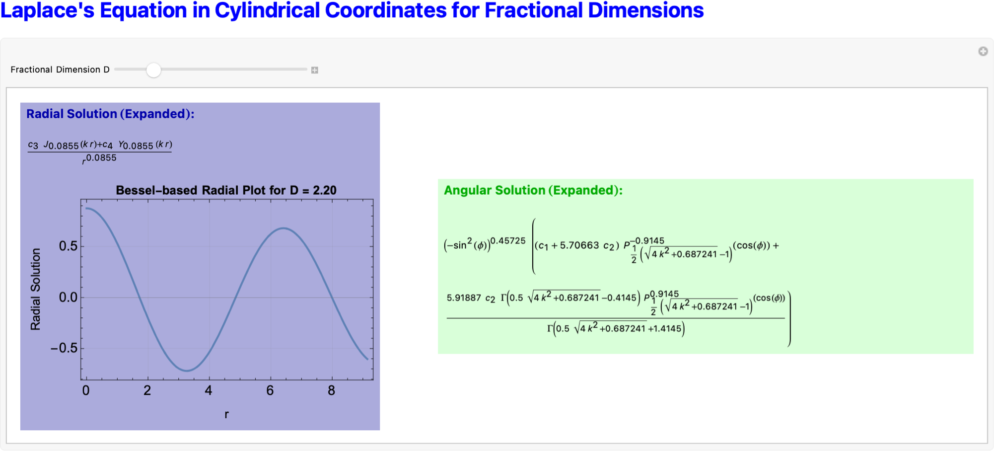
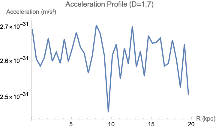
Also we mustn't forget to model how wavefunctions, potentials, and gravitational-like forces behave in fractional-dimensional cylindrical spaces, where the dimension D is allowed to scale between 2 and 3. So we can demonstrate some fractional radial solutions using Bessel functions and Gegenbauer polynomials to describe the radial and angular behavior of fields and waves. These solutions plus exponential decay along the vertical axis make for some formidable, full 3D potentials for almost any wavefunction. The gravitational potential is a modular, surface mass density profile, and its dimensional variation...is in relation to our computed acceleration profiles based on the derived fractional potentials, helping to illustrate how gravitational forces would look in lower-dimensional or fractal-like settings. With the power of Mathematica, in real-time let's go exploring how the radial and angular structures evolve as the dimension D changes, focusing on features such as radial spread, angular localization, and attenuation along the vertical direction. In conclusion, the underlying spatial dimension has quite an effect on wave propagation & gravitational behavior, that's the connection to theoretical studies in photon transport, gravitational modeling, and fractional field theories.
ClearAll["Global`*"];
radialSolution[D_, k_,
R_] := (k R)^((3 - D)/2) BesselJ[(D - 3)/2, k R];
FractionalCylindricalSolution[R_, \[Phi]_, z_, D_, k_, m_] :=
Module[{\[Lambda], radial, angular, vertical}, \[Alpha]z = 1;
\[Lambda] = (D - \[Alpha]z - 2)/2;
radial = (k R)^((3 - D)/2) BesselJ[\[Lambda] + m, k R];
angular = GegenbauerC[m, \[Lambda], Cos[\[Phi]]];
vertical = Exp[-k Abs[z]];
radial*angular*vertical];
standardSolution[R_, k_] := BesselJ[0, k R];
Manipulate[
Module[{fractional, standard},
fractional = FractionalCylindricalSolution[R, 0, 0, D, 1, 0];
standard = standardSolution[R, 1];
Show[Plot[{fractional, standard}, {R, 0, 5},
PlotStyle -> {Thick, {Dashed, Red}},
PlotLegends ->
Placed[{Style[
"Fractional Solution (D = " <>
ToString@NumberForm[D, {2, 2}] <> ")", Black],
Style["Standard Solution (D = 3)", Red]}, Above],
Frame -> True,
FrameLabel -> {"Radial Distance R", "Potential \[CapitalPhi](R)"},
FrameStyle -> Directive[Black, 14], LabelStyle -> {Black, 12},
ImageSize -> Large, PlotRange -> All, GridLines -> Automatic],
PlotLabel ->
Style["Comparison of Fractional and Standard Laplace Solutions",
Bold, 16]]], {{D, 2.5, "Fractional Dimension D"}, 1.0, 3.0, 0.05,
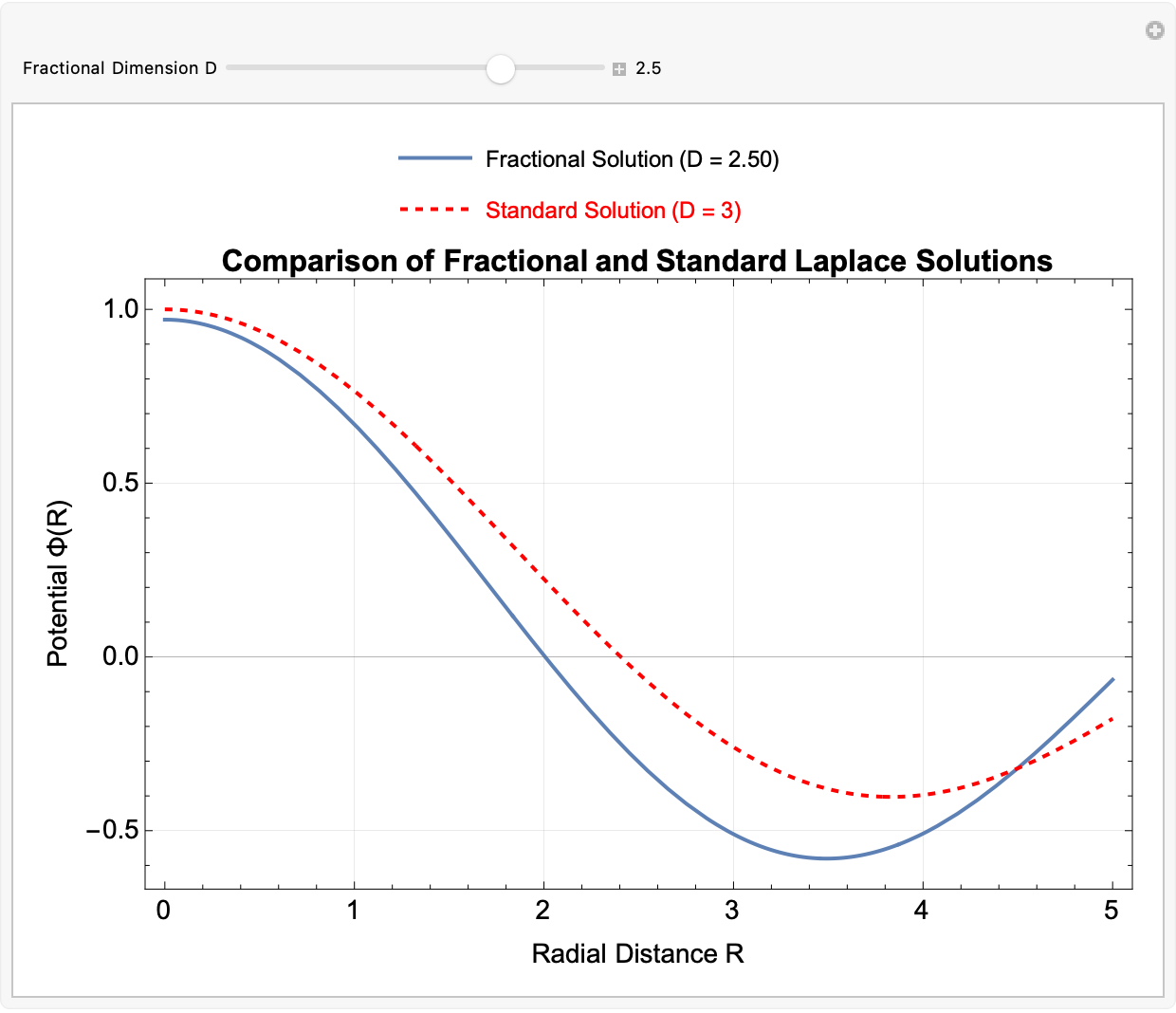
Appearance -> "Labeled"}, SaveDefinitions -> True]
ClearAll["Global`*"];
safeR[r_] := Max[r, 10^-6];
safePhi[\[Phi]_] :=
  Which[Abs[Mod[\[Phi], \[Pi]] - \[Pi]/2] < 10^-6, \[Pi]/2 + 10^-6,
   Abs[Mod[\[Phi], \[Pi]] + \[Pi]/2] < 10^-6, -(\[Pi]/2) + 10^-6,
   True, \[Phi]];
FractionalCylindricalLaplacian[\[Psi]_, r_, \[Phi]_, z_, D_] :=
  Module[{rr, pp}, rr = safeR[r];
   pp = safePhi[\[Phi]];
   (1/rr^(D - 2))  D[rr^(D - 2) D[\[Psi], r],
      r] + (1/rr^2) D[\[Psi], {\[Phi], 2}] +
    D[\[Psi], {z, 2}] + (D - 3)/(rr^2 Tan[pp]) D[\[Psi], \[Phi]]];
RadialSolution[r_, k_, D_] :=
  safeR[r]^((3 - D)/2) BesselJ[(D - 3)/2, k*safeR[r]];
AngularSolution[\[Phi]_, m_, D_] :=
  GegenbauerC[m, (D - 3)/2, Cos[safePhi[\[Phi]]]];
AxialSolution[z_, kz_] := Exp[-kz Abs[z]];
WaveSolution[r_, \[Phi]_, z_, k_, kz_, m_, D_] :=
  RadialSolution[r, k, D]*AngularSolution[\[Phi], m, D]*
   AxialSolution[z, kz];
Manipulate[Module[{sol}, sol = WaveSolution[r, \[Phi], 0, k, kz, m, D];
  ListPlot3D[
   Flatten[Table[{r*Cos[\[Phi]], r*Sin[\[Phi]],
      Re[sol /. {r -> r, \[Phi] -> \[Phi], k -> k, m -> m}]}, {r,
      0.01, 1, 0.05}, {\[Phi], 0, 2 \[Pi], \[Pi]/20}], 1],
   ColorFunction -> "Rainbow", PlotRange -> All,
   AxesLabel -> {"X", "Y", "\[CapitalPsi]"},
   PlotLabel -> StringForm["Fractional Dimension D = ``", D]]], {{D,
   2.5, "Dimension"}, 2, 3, 0.1,
  Appearance -> "Labeled"}, {{k, 1, "Radial Wave Number"}, 0.5, 5,
  0.1, Appearance -> "Labeled"}, {{m, 0, "Angular Mode"}, 0, 5, 1,
  Appearance -> "Labeled"}, {{kz, 0, "Axial Wave Number"}, 0, 5, 0.1,
  Appearance -> "Labeled"}, {{plotType, "3D", "Plot Type"}, {"3D"}},
 ControlPlacement -> Left]
Plot3D[Re[
  WaveSolution[Sqrt[x^2 + y^2], ArcTan[x, y], 0, 1, 0, 1,
   2.5]], {x, -1, 1}, {y, -1, 1}, ColorFunction -> "Rainbow",
 AxesLabel -> {"X", "Y", "\[CapitalPsi]"},
 PlotLabel -> "Cylindrical Wave in D=2.5 Space"]
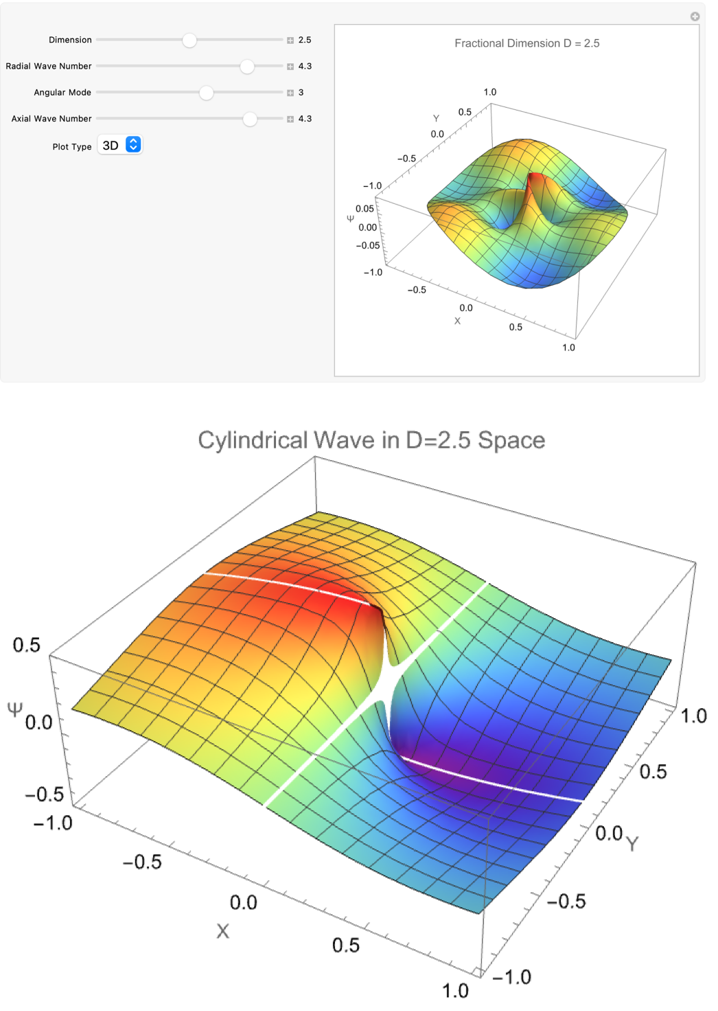
How do fractional-dimensional cylindrical spaces differ from the familiar standard three-dimensional case? Well, we've already built a fractional generalization of Laplace's equation, constructing radial solutions with Bessel functions and angular solutions with Gegenbauer polynomials, all non-integer dimensions considered..we compare the fractional solution to the standard D = 3 solution, to show how the field's radial behavior tightens or spreads depending on the space's dimensionality. A separate part constructs complete 3D wavefunctions that include radial, angular, and vertical decay components, using safe handling of singularities near r = 0 and critical angular points. Therefore the wave profile changes as the dimension D, radial wave number k, angular mode m, and axial wave number k vary. So fractional-dimensional geometry dramatically alters wave propagation, not just in photonic fields but also in exotic or effective lower-dimensional spaces.
ClearAll["Global`*"];
FractionalLaplacianCylindrical[D_, f_, r_, \[Phi]_, z_] :=
  Module[{\[Alpha]r = D - 2, \[Alpha]\[Phi] = 1, \[Alpha]z =
     1}, (1/r^\[Alpha]r D[r^\[Alpha]r D[f, r],
       r] + (1/(r^2 Sin[\[Phi]]^(D - 3)) D[
         Sin[\[Phi]]^(D - 3) D[f, \[Phi]], \[Phi]] + D[f, {z, 2}]))];
FractionalWaveSolution[D_, r_, \[Phi]_, z_, k_, m_] :=
  Module[{radialPart = (k r)^((3 - D)/2) BesselJ[(D - 3)/2 + m, k r],
    angularPart = GegenbauerC[m, (D - 3)/2, Cos[\[Phi]]],
    verticalPart = Exp[-k Abs[z]]},
   radialPart*angularPart*verticalPart];
Manipulate[
 Module[{sol, coordinates},
  sol = FractionalWaveSolution[D, r, \[Phi], 0, 1, 0];
  coordinates =
   Table[{r Cos[\[Phi]], r Sin[\[Phi]], sol}, {r, 0.1, 5,
     0.2}, {\[Phi], 0, 2 \[Pi], \[Pi]/20}];
  ListPlot3D[Flatten[coordinates, 1], ColorFunction -> "Rainbow",
   PlotRange -> All, AxesLabel -> {"X", "Y", "Amplitude"},
   PlotLabel -> StringForm["D=`` Cylindrical Wave", D],
   MeshFunctions -> {#3 &}, Mesh -> 10]], {{D, 2.5,
   "Fractional Dimension"}, 2, 3, 0.1, Appearance -> "Labeled"},
 TrackedSymbols :> {D}]
radialSolution[D_, k_, R_] := (k*R)^((3 - D)/2)*BesselJ[(D - 3)/2, k*R]
Manipulate[
 Plot[radialSolution[D, k, R], {R, 0, 10}, PlotRange -> All,
  AxesLabel -> {"Radial Distance R", "Amplitude"},
  PlotLabel ->
   Style[Row[{"Dimension D = ", D, ", Wave Number k = ", k}], 14,
    Bold], ImageSize -> 500, PlotStyle -> {Thick, ColorData[97, 1]},
  GridLines -> Automatic,
  GridLinesStyle -> LightGray], {{D, 3, "Dimension D"}, 2, 3, 0.1,
  Appearance -> "Labeled"}, {{k, 1, "Wave Number k"}, 0.1, 2, 0.1,
  Appearance -> "Labeled"}, ControlPlacement -> Left,
 TrackedSymbols :> {D, k}]
ClearAll["Global`*"];
radialEquation = J''[R] + ((D - 2)/R) J'[R] + k^2 J[R] == 0;
radialSolution = DSolve[radialEquation, J[R], R];
radialFunction = J[R] /. radialSolution[[1]];
k = 1;
dimensions = Range[2.1, 3, 0.1];
Plot3D[radialFunction /. {C[1] -> 1, C[2] -> 0, k -> 1}, {R, 0,
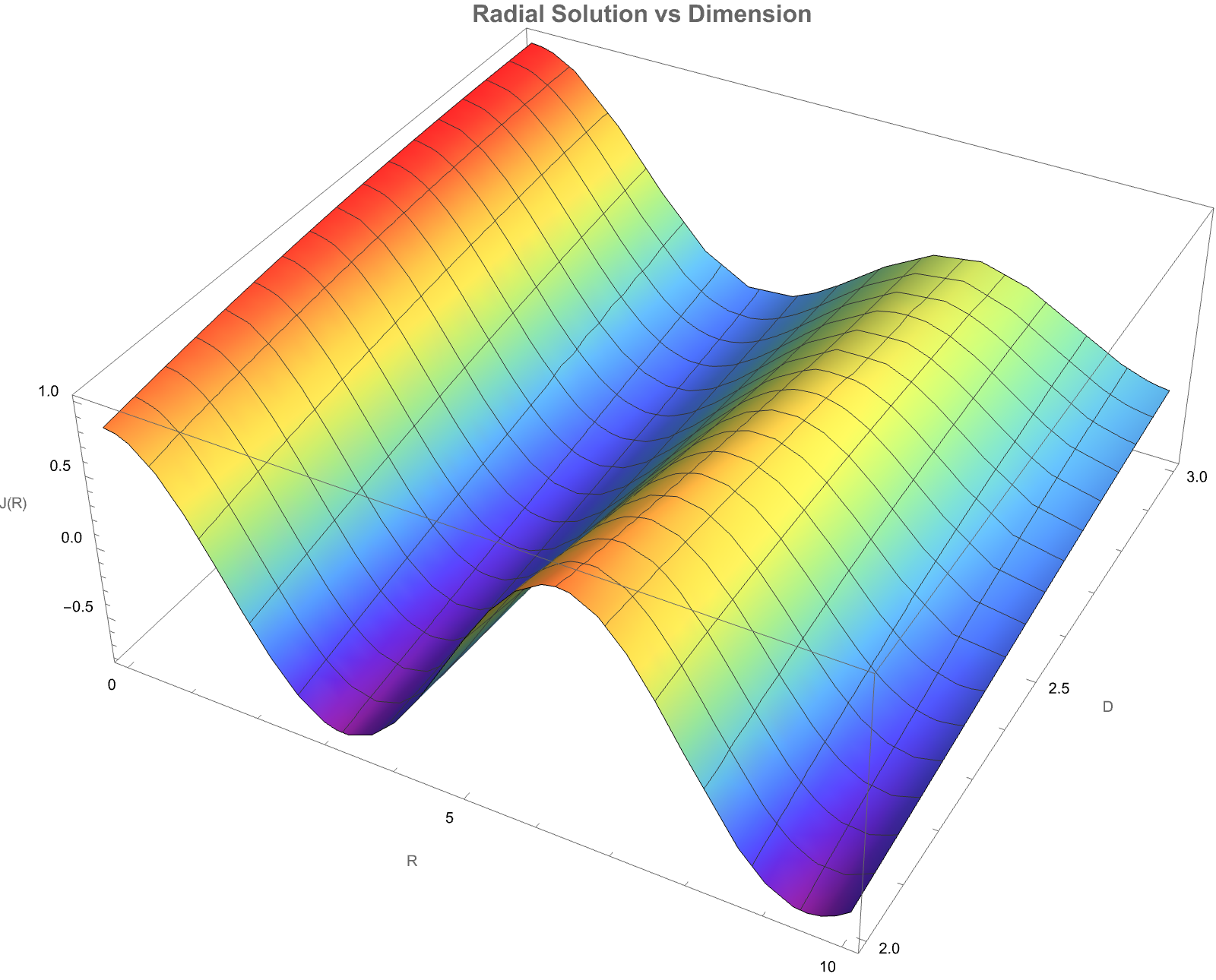
10}, {D, 2, 3}, AxesLabel -> {"R", "D", "J(R)"},
PlotLabel -> Style["Radial Solution vs Dimension", 16, Bold],
ColorFunction -> "Rainbow", ImageSize -> 800]
ClearAll["Global`*"];
FractionalCylindricalLaplacian[\[Psi]_, R_, \[Phi]_, z_, D_] :=
Module[{},
1/R^(D - 2)*D[R^(D - 2)*D[\[Psi], R], R] +
1/(R^2*Sin[\[Phi]]^(D - 3))*
D[Sin[\[Phi]]^(D - 3)*D[\[Psi], \[Phi]], \[Phi]] +
D[\[Psi], {z, 2}]]
\[CapitalPsi][R_, \[Phi]_, z_] :=
Rradial[R]*Rangular[\[Phi]]*Exp[-k*Abs[z]]
Rangular[\[Phi]_] := GegenbauerC[m, (Ddim - 3)/2, Cos[\[Phi]]]
Rradial[R_] := (k*R)^((3 - Ddim)/2)*BesselJ[(Ddim - 3)/2 + m, k*R]
Ddim = 4.5;
m = 0;
k = 1;
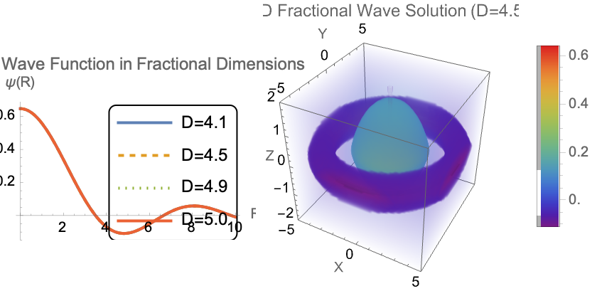
RadialPlot =
Plot[Evaluate@
Table[Rradial[R] /. {Ddim -> d, m -> 0, k -> 1}, {d, {4.1, 4.5,
4.9, 5.0}}], {R, 0, 10},
PlotStyle -> {Thick, Dashed, Dotted, Thick},
PlotLegends ->
Placed[LineLegend[{"D=4.1", "D=4.5", "D=4.9", "D=5.0"},
LegendFunction -> "Frame"], {Right, Top}],
AxesLabel -> {"R", "\[Psi](R)"},
PlotLabel -> "Radial Wave Function in Fractional Dimensions"];
WavePlot3D =
DensityPlot3D[
Evaluate[\[CapitalPsi][Sqrt[x^2 + y^2], ArcTan[x, y],
z] /. {Ddim -> 4.5, m -> 0, k -> 1}], {x, -5, 5}, {y, -5,
5}, {z, -2, 2}, PlotLegends -> Automatic,
ColorFunction -> "Rainbow",
PlotLabel -> "3D Fractional Wave Solution (D=4.5)",
AxesLabel -> {"X", "Y", "Z"}];
Grid[{{RadialPlot, WavePlot3D}}]
ClearAll["Global`*"];
FractionalCylindricalLaplacian[D_][f_, r_, \[Phi]_, z_] :=
  Module[{\[Alpha]r = D - 2, \[Alpha]\[Phi] = 1, \[Alpha]z =
     1}, (1/r^\[Alpha]r)*D[r^\[Alpha]r*D[f, r], r] + (1/r^2)*
     D[f, {\[Phi], 2}] + D[f, {z, 2}]];
FractionalCylindricalWaveSolution[D_, k_, m_, n_, r_, \[Phi]_, z_,
   t_] := Module[{radialPart, angularPart, zPart, timePart},
   radialPart = BesselJ[(D - 3)/2 + m, k*r];
   angularPart = Exp[I*m*\[Phi]];
   zPart = Exp[-k*Abs[z]];
   timePart = Exp[I*Sqrt[k^2 - n^2]*t];
   radialPart*angularPart*zPart*timePart];
DValue = 2.5;
kValue = 1;
mValue = 0;
Manipulate[
 Module[{wave, coordinates},
  wave = FractionalCylindricalWaveSolution[D, k, m, 0, r, \[Phi], 0,
    t];
  coordinates =
   Table[{r*Cos[\[Phi]], r*Sin[\[Phi]], Re[wave]}, {r, 0.1, 5,
     0.5}, {\[Phi], 0, 2 \[Pi], \[Pi]/20}];
  ListPlot3D[Flatten[coordinates, 1], ColorFunction -> "Rainbow",
   PlotRange -> All, AxesLabel -> {"X", "Y", "Amplitude"},
   PlotLabel -> StringForm["D=``, k=``, m=``", D, k, m]]], {{D, 2.5,
   "Dimension"}, 2.1, 2.9, 0.1,
  Appearance -> "Labeled"}, {{k, 1, "Wave Number"}, 0.5, 2, 0.1,
  Appearance -> "Labeled"}, {{m, 0, "Azimuthal Mode"}, 0, 2, 1,
  Appearance -> "Labeled"}, {t, 0, 2 \[Pi], AnimationRate -> 0.5}]
Plot3D[Re[
  FractionalCylindricalWaveSolution[0, 1, 0, 0, Sqrt[x^2 + y^2],
   ArcTan[x, y], 0, 0]], {x, -5, 5}, {y, -5, 5},
 ColorFunction -> "Aquamarine", PlotRange -> All,
 AxesLabel -> {"X", "Y", "Amplitude"},
 PlotLabel -> "Fractional Cylindrical Wave (D=0)"]
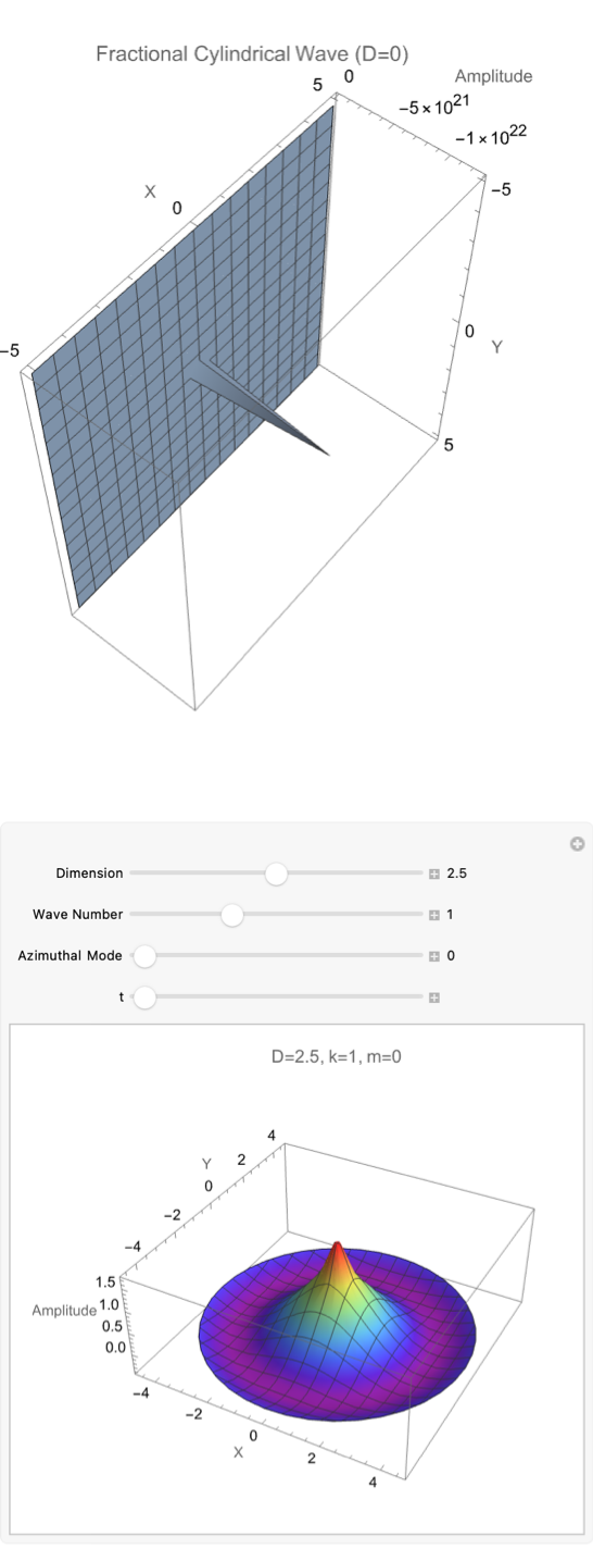
RadialSolution[D_, m_, k_,
  R_] := (k R)^((3 - D)/2) BesselJ[(D - 3)/2 + m, k R]
VerticalSolution[k_, z_] := Exp[-k Abs[z]]
FullSolution[D_, k_, R_, z_] :=
 RadialSolution[D, 0, k, R]*VerticalSolution[k, z]
Manipulate[
 Plot3D[FullSolution[D, k, R, z], {R, 0.1, 10}, {z, -5, 5},
  PlotLabel ->
   Row[{"Fractional Cylindrical Wave\nDimension D = ", D}],
  AxesLabel -> {"R", "z", "\[CapitalPhi](R,z)"},
  ColorFunction -> "TemperatureMap", MeshFunctions -> {#3 &},
  PlotRange -> All,
  PerformanceGoal -> "Quality"], {{D, 2.5, "Dimension"}, 1, 3, 0.1,
  Appearance -> "Labeled"}, {{k, 0.5, "Wave Number"}, 0.1, 2, 0.1,
  Appearance -> "Labeled"}, ControlPlacement -> Left]
DensityPlot[FullSolution[2.5, 0.7, R, z], {R, 0.1, 10}, {z, -5, 5},
 PlotLabel -> "Potential Distribution (D=2.5, k=0.7)",
 FrameLabel -> {"R", "z"}, ColorFunction -> "SunsetColors",
 PlotLegends -> Automatic]
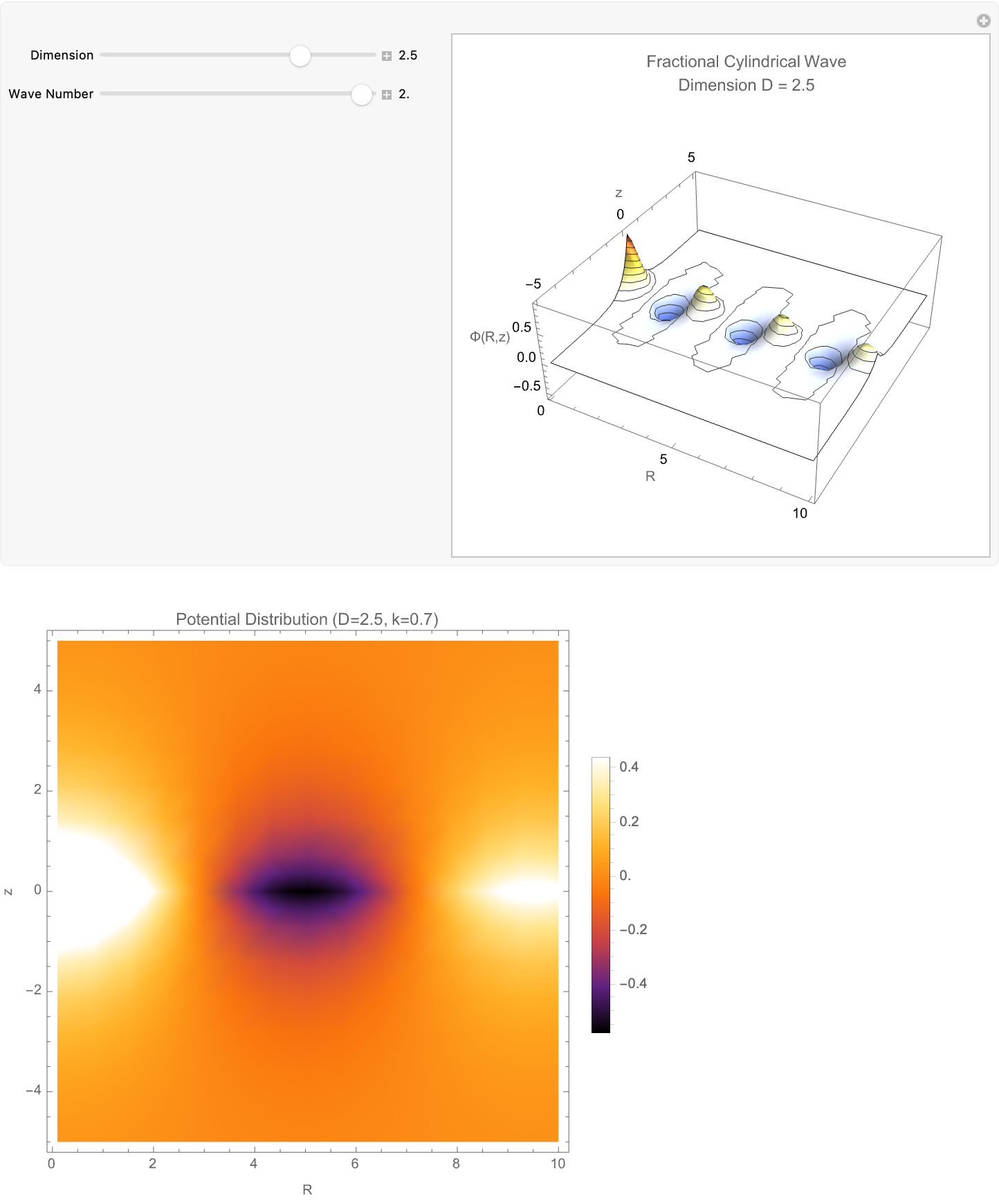
ClearAll["Global`*"];
FractionalLaplacianCylindrical[\[CapitalPhi]_, R_, \[Phi]_, z_, D_] :=
  Module[{},
  1/R^(D - 2)*D[R^(D - 2)*D[\[CapitalPhi], R], R] +
   1/(R^2*Sin[\[Phi]]^(D - 3))*
    D[Sin[\[Phi]]^(D - 3)*D[\[CapitalPhi], \[Phi]], \[Phi]] +
   D[\[CapitalPhi], {z, 2}]]
SolutionForm[R_, z_, \[Phi]_, D_, k_, m_] := (k*R)^((3 - D)/2)*
  BesselJ[(D - 3)/2 + m, k*R]*GegenbauerC[m, (D - 3)/2, Cos[\[Phi]]]*
  Exp[-k*Abs[z]]
DValue = 0.7;
kValue = 0.1;
mValue = 0;
Potential[R_, z_, \[Phi]_] :=
 SolutionForm[R, z, \[Phi], DValue, kValue, mValue]
DensityPlot3D[
 Potential[Sqrt[x^2 + y^2], z, ArcTan[x, y]], {x, -15, 15}, {y, -15,
  15}, {z, -2, 2}, PlotLegends -> Automatic,
 ColorFunction -> "Rainbow", PlotRange -> All,
 AxesLabel -> {"X (kpc)", "Y (kpc)", "Z (kpc)"},
 PlotLabel ->
  Style["Fractional-Dimensional Gravitational Potential (D=0.7)", 12,
   Bold]]
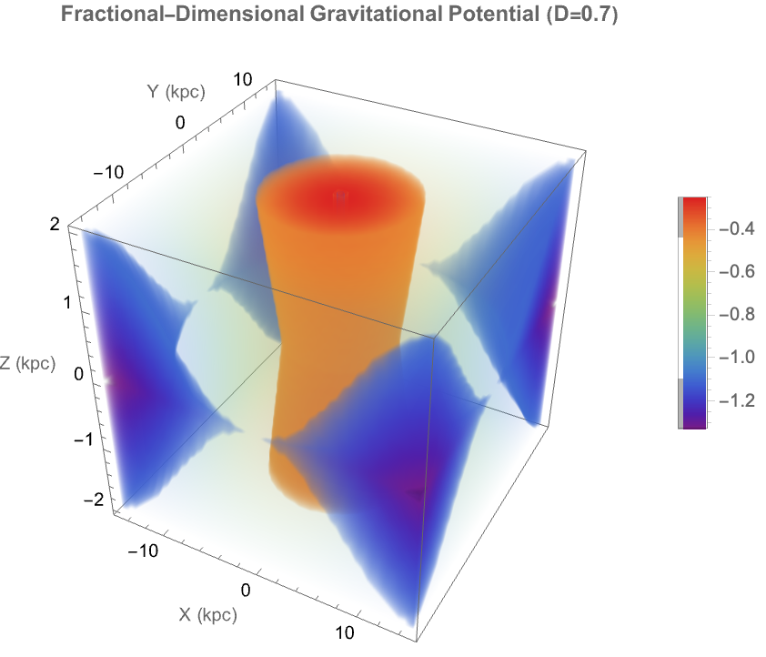
ClearAll["Global`*"];
DVal = 2.5;
k = 1;
c = 1;
m = 0;
radialEquation =
  R''[r] + ((DVal - 2)/r) R'[r] + (k^2 - m^2/r^2) R[r] == 0;
radialSolution = DSolve[radialEquation, R[r], r] // Simplify;
RSolution[r_] = radialSolution[[1, 1, 2]] /. {C[1] -> 1, C[2] -> 0}
FPhi[\[CurlyPhi]_] = 1;
TSolution[t_] = Exp[-I c k t];
Phi[r_, \[CurlyPhi]_, t_] =
  RSolution[r]*FPhi[\[CurlyPhi]]*Re[TSolution[t]];
Animate[Plot[Phi[r, 0, t], {r, 0.1, 10},
  PlotRange -> {{0, 10}, {-1.2, 1.2}},
  PlotLabel ->
   Style["Radial Wave Profile at t = " <> ToString[t] <> " (D = " <>
     ToString[DVal] <> ")", 14],
  AxesLabel -> {"Radius (r)", "Amplitude"}], {t, 0,
  2 \[Pi], \[Pi]/10}]
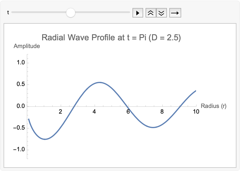
Manipulate[
 Module[{k = 1, radialSolution, angularSolution, combinedSolution},
  radialSolution[r_] := (k*r)^((3 - dim)/2)*
    BesselJ[(dim - 3)/2 + m, k*r];
  angularSolution[\[CurlyPhi]_] :=
   GegenbauerC[m, (dim - 3)/2, Cos[\[CurlyPhi]]];
  PolarPlot[
   radialSolution[r]*angularSolution[\[CurlyPhi]] /. \[CurlyPhi] ->
     0, {r, 0, 10}, PlotRange -> All, AxesLabel -> {"R", "Amplitude"},
    PlotLabel ->
    Style[Row[{"Fractional Cylindrical Wave Solution\n",
       "Dimension D = ", NumberForm[dim, {3, 1}], ", Mode m = ", m}],
     14, Bold], ImageSize -> 500,
   PlotStyle -> ColorData["Rainbow"][(dim - 1)/2],
   GridLines -> Automatic, GridLinesStyle -> LightGray]], {{dim, 2.0,
   "Space Dimension (D)"}, 1.1, 2.9, 0.1,
  Appearance -> "Labeled"}, {{m, 0, "Azimuthal Mode Number"}, 0, 3, 1,
   Appearance -> "Labeled"}, TrackedSymbols :> {dim, m},
 ControlPlacement -> Left, Paneled -> True,
 FrameLabel -> Style["Fractional Space Wave Solutions", 14, Bold]]
DValue = 2.5;
k = 1;
omega = 1;
c = 1;
radialSolutionD[r_] := (k*r)^((3 - DValue)/2)*
  BesselJ[(DValue - 3)/2, k*r]
radialSolution3D[r_] := BesselJ[0, k*r]
timeSolution[t_] := Exp[-I*omega*t]
waveFunction[r_, t_, D_] :=
 Module[{radial},
  radial = If[D == 3, radialSolution3D[r], radialSolutionD[r]];
  radial*timeSolution[t]]
Plot[{Abs[radialSolutionD[r]], Abs[radialSolution3D[r]]}, {r, 0, 10},
 PlotStyle -> {Blue, Red}, PlotLegends -> {"D=2.5", "D=3"},
 AxesLabel -> {"Radial Distance (R)", "Amplitude"},
 PlotLabel -> "Radial Wave Solutions Comparison", BaseStyle -> 14]
Plot3D[Re[waveFunction[r, t, 2.5]], {r, 0, 10}, {t, 0, 10},
 AxesLabel -> {"R", "Time", "Re[\[Psi]]"},
 PlotLabel -> "Cylindrical Wave in D=2.5 Space",
 ColorFunction -> "Rainbow", MeshFunctions -> {#3 &}, BaseStyle -> 14]
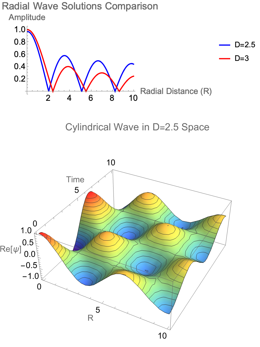
d = 2.5;
k = 1;
radialSolution[r_] := r^((2 - d)/2)*BesselI[(d - 2)/2, k*r]
zSolution[z_] := Exp[-k*z]
potential[r_, z_] := radialSolution[r]*zSolution[z]
Plot3D[potential[r, z], {r, 0.1, 5}, {z, 0, 5}, PlotRange -> All,
 AxesLabel -> {"R", "Z", "\[CapitalPhi]"},
 PlotLabel -> StringForm["Fractional Laplace Equation (D=``)", d],
 ColorFunction -> "TemperatureMap"]
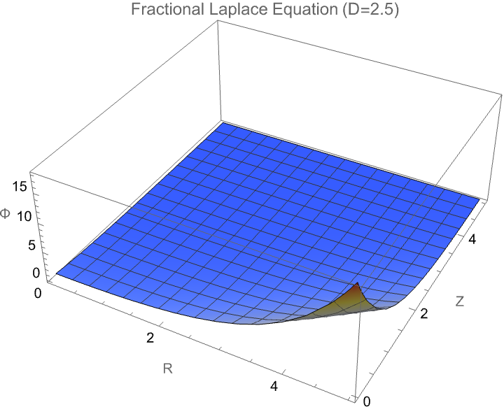
ClearAll["Global`*"];
Off[Power::indet];
Manipulate[
 Module[{\[Nu], \[Mu], RSol, ZSol}, \[Nu] =
   Sqrt[((2 - 1 - 1)/2)^2 + m^2];
  RSol[\[Rho]_] := \[Rho]^0*(BesselJ[\[Nu], \[Beta]\[Rho]  \[Rho]] +
      BesselY[\[Nu], \[Beta]\[Rho]  \[Rho]]);
  RSol[0] = Limit[RSol[\[Rho]], \[Rho] -> 0];
  \[CapitalPhi][\[Theta]_] := Cos[m  \[Theta]];
  \[Mu] = (1 - \[Alpha]3)/2;
  ZSol[z_] :=
   z^((1 - \[Alpha]3)/2)  (BesselJ[\[Mu], \[Beta]z  z] +
      BesselY[\[Mu], \[Beta]z  z]);
  ZSol[0] = Limit[ZSol[z], z -> 0];
  Column[{Plot[RSol[\[Rho]], {\[Rho], 0.1, 10},
     AxesLabel -> {"\[Rho]", "R(\[Rho])"}, PlotLabel -> "Radial"],
    Plot[\[CapitalPhi][\[Theta]], {\[Theta], 0, 2  \[Pi]},
     AxesLabel -> {"\[Theta]", "\[CapitalPhi](\[Theta])"},
     PlotLabel -> "Angular"],
    Plot[ZSol[z], {z, 0.1, 10}, AxesLabel -> {"z", "Z(z)"},
     PlotLabel -> "Longitudinal"]}]], {{m, 0, "m"}, 0, 5, 1,
  Appearance -> "Labeled"}, {{\[Alpha]3, 1, "\[Alpha]3"}, 0.1, 1,
  Appearance -> "Labeled"}, {{\[Beta]\[Rho], 1, "\[Beta]\[Rho]"}, 0,
  2, Appearance -> "Labeled"}, {{\[Beta]z, 1, "\[Beta]z"}, 0, 2,
  Appearance -> "Labeled"},
 TrackedSymbols :> {m, \[Alpha]3, \[Beta]\[Rho], \[Beta]z}]
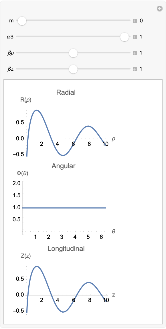
Here you will find fractional-dimensional cylindrical waves and gravitational potentials, where space has a non-integer dimension D. By solving modified Laplacian and Helmholtz equations, we show how radial spread, angular localization, and vertical decay are altered compared to standard three-dimensional behavior. The simulations resurface the old wave and field structures relevant to photon propagation, fractal media, and new gravity theories.
ClearAll["Global`*"];
Ddim = 2.5;
k = 1;
radialODE = J''[R] + (Ddim - 2)/R J'[R] + k^2 J[R] == 0;
radialSol = DSolve[radialODE, J[R], R];
radialSolution = J[R] /. radialSol[[1]];
verticalODE = Z''[z] - k^2 Z[z] == 0;
verticalSol = DSolve[verticalODE, Z[z], z];
verticalSolution = Z[z] /. verticalSol[[1]];
potential[R_, z_] = radialSolution*verticalSolution;
visualizationSolution =
  potential[R, z] /. {C[1] -> 1, C[2] -> 0, C[3] -> 1, C[4] -> 0};
Plot3D[Evaluate[visualizationSolution], {R, 0, 5}, {z, -5, 5},
 PlotRange -> All, ColorFunction -> "TemperatureMap",
 AxesLabel -> {"R", "z", "\[CapitalPhi](R,z)"},
 PlotLabel ->
  StringForm["Fractional-Dimensional Potential (D=``)", Ddim],
 MeshFunctions -> {#3 &}, Mesh -> 20, PerformanceGoal -> "Quality"]
ContourPlot[Evaluate[visualizationSolution], {R, 0, 5}, {z, -5, 5},
 FrameLabel -> {"R", "z"}, PlotLegends -> Automatic,
 ColorFunction -> "ThermometerColors", Contours -> 20,
 PlotLabel -> StringForm["Potential Contours (D=``)", Ddim]]
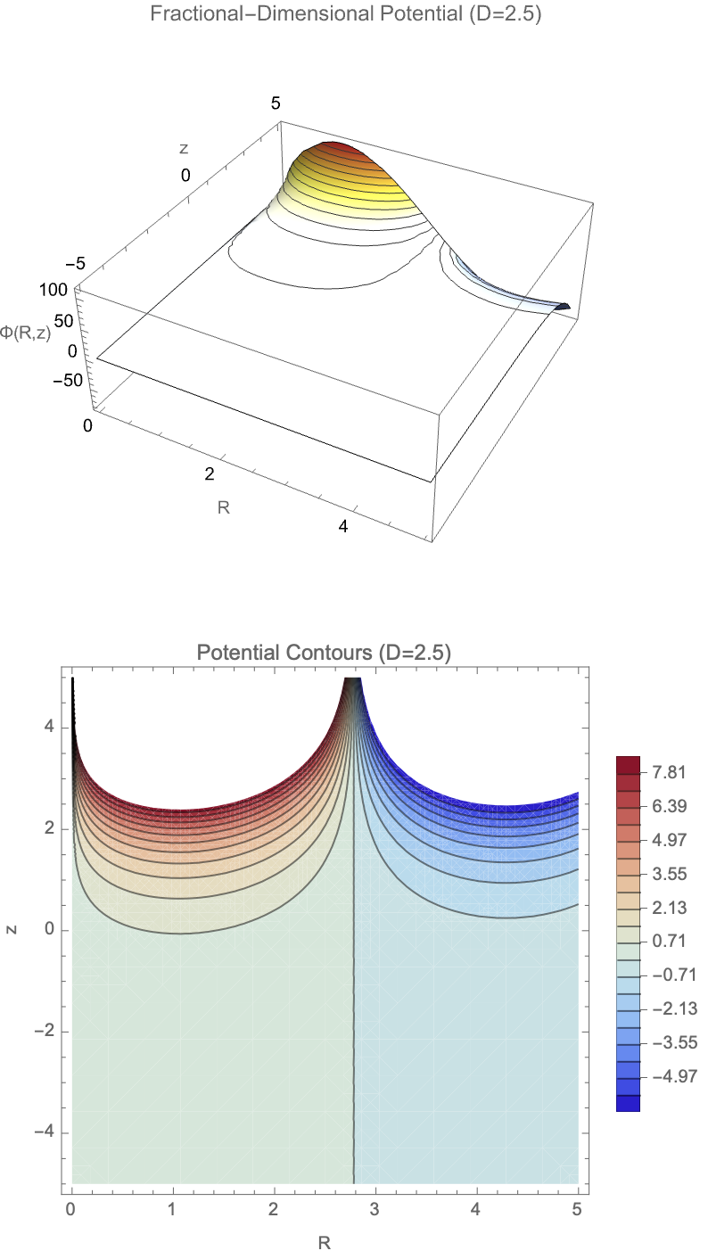
ClearAll["Global`*"];
FractionalLaplacianCylindrical[D_, f_, r_, \[Phi]_, z_] :=
  Module[{},
   1/r^(D - 2) D[r^(D - 2) D[f, r], r] +
    1/(r^2 Sin[\[Phi]]^(D - 3)) D[
      Sin[\[Phi]]^(D - 3) D[f, \[Phi]], \[Phi]] + D[f, {z, 2}]];
FractionalHelmholtz[\[Psi]_, k_, D_, r_, \[Phi]_, z_] :=
  FractionalLaplacianCylindrical[D, \[Psi][r, \[Phi], z], r, \[Phi],
     z] + k^2 \[Psi][r, \[Phi], z] == 0;
\[Psi]Solution[r_, \[Phi]_, z_, D_, m_, kz_, n_] :=
  Module[{kr =
     Sqrt[k^2 - kz^2]}, (BesselJ[(D - 3)/2 + m, kr r]/r^((D - 3)/2)*
     GegenbauerC[n, (D - 3)/2, Cos[\[Phi]]]*Exp[-kz Abs[z]])];
k = 1;
m = 0;
kz = 0.5;
n = 0;
Manipulate[
 Module[{D = dim, kr = Sqrt[k^2 - kzVal^2]},
  DensityPlot3D[
   BesselJ[(D - 3)/2, kr r]/r^((D - 3)/2)*Cos[\[Phi]]*
    Exp[-kzVal Abs[z]], {r, 0, 10}, {\[Phi], 0, 2 \[Pi]}, {z, -2, 2},
   PlotLabel -> Row[{"Fractional Dimension D = ", dim}],
   ColorFunction -> "TemperatureMap",
   BoxRatios -> {1, 1, 0.5}]], {{dim, 2.5, "Dimension D"}, 2.1, 3,
  0.1, Appearance -> "Labeled"}, {{kzVal, 0.5,
   "Vertical Wave Number kz"}, 0, 1, 0.1, Appearance -> "Labeled"}]
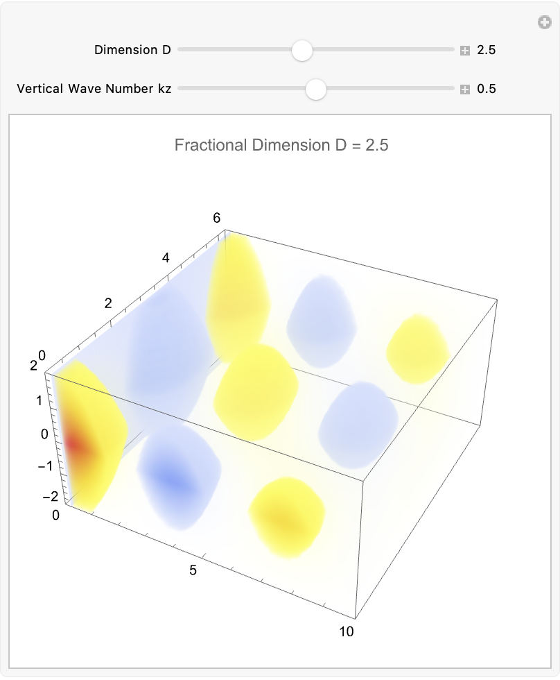
ClearAll["Global`*"];
FractionalLaplacianCylindrical[\[Psi]_, R_, \[CurlyPhi]_, z_, D_] :=
 1/R^(D - 2)  D[R^(D - 2)  D[\[Psi], R], R] +
  1/(R^2  Sin[\[CurlyPhi]]^(D - 3))  D[
    Sin[\[CurlyPhi]]^(D - 3)  D[\[Psi], \[CurlyPhi]], \[CurlyPhi]] +
  D[\[Psi], {z, 2}]
FractionalWaveSolution[R_, \[CurlyPhi]_, z_, D_, k_, m_] :=
 Module[{\[Nu] = (3 - D)/2 + m, \[Lambda] = (D - 3)/2},
  radial = (k  R)^((3 - D)/2)  BesselJ[\[Nu], k  R];
  angular = GegenbauerC[m, \[Lambda], Cos[\[CurlyPhi]]];
  vertical = Exp[-k  Abs[z]];
  radial*angular*vertical]
Dvals = {2.0, 2.5, 3.0};
k = 0.1;
m = 0;
z0 = 0;
colors = ColorData["Rainbow"] /@ Rescale[Dvals];
labels = ("D = " <> ToString[#]) & /@ Dvals;
curves =
  Table[FractionalWaveSolution[R, 0, z0, D, k, m], {D, Dvals}];
D25Wave[R_, \[CurlyPhi]_] :=
  FractionalWaveSolution[R, \[CurlyPhi], z0, 2.5, k, m];
sphPlot =
 SphericalPlot3D[
  D25Wave[r, \[CurlyPhi]], {r, 0, 20}, {\[CurlyPhi], 0, 2  \[Pi]},
  PlotTheme -> "Detailed", Mesh -> None,
  ColorFunction ->
   Function[{x, y, z, th, ph}, ColorData["Thermometer"][z]],
  ColorFunctionScaling -> True, Lighting -> "Neutral", Boxed -> False,
   Axes -> False, ImageSize -> 450,
  PlotLabel ->
   Style["Wave Pattern in D = 2.5 Fractal Space", 16, Bold]]
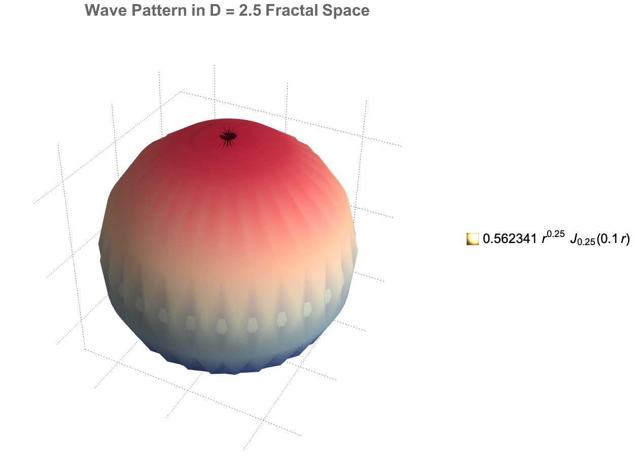
ClearAll[RadialSolution];
RadialSolution[r_, D_, k_,
  m_] := (k  r)^((3 - D)/2)  BesselJ[(D - 3)/2 + m, k  r]
k = 1; m = 0;
dims = Range[2, 3, 0.2];
colors = ColorData["BrightBands"] /@ Rescale[dims];
Plot[Evaluate@Table[RadialSolution[r, D, k, m], {D, dims}], {r, 0.1,
  10}, PlotTheme -> "Detailed",
 PlotStyle -> Map[{#, Thick} &, colors],
 PlotLegends ->
  Placed[LineLegend[colors, ("D = " <> ToString[#]) & /@ dims,
    LegendLabel -> "Dimension"], Below], Frame -> True,
 FrameLabel -> (Style[#, 14, Bold] & /@ {"r", "R(r)"}),
 FrameTicksStyle -> Directive[FontSize -> 12], GridLines -> Automatic,
  ImageSize -> Medium,
 PlotLabel -> Style["Radial Wave Solutions for Varying D", 16, Bold]]
Manipulate[
 Plot[RadialSolution[r, D, k, m], {r, 0.1, 10},
  PlotTheme -> "Detailed",
  PlotStyle -> {Thick, ColorData["DarkRainbow"][Rescale[D, {2, 3}]]},
  Frame -> True,
  FrameLabel -> (Style[#, 14, Bold] & /@ {"r", "R(r)"}),
  FrameTicksStyle -> Directive[FontSize -> 12], PlotRange -> All,
  ImageSize -> Medium,
  PlotLabel ->
   Style["Radial Solution, D = " <> ToString[NumberForm[D, {2, 1}]],
    16, Bold]], {{D, 2.5, "Dimension D"}, 2, 3, 0.1,
  Appearance -> "Labeled"}]
\[Omega] = 1;
\[Psi][r_, t_, D_] := RadialSolution[r, D, k, m]*Cos[\[Omega]  t];
Animate[Plot[\[Psi][r, t, 2.5], {r, 0.1, 10}, PlotTheme -> "Detailed",
   PlotStyle -> {Thick, ColorData["TemperatureMap"][0.8]},
  Frame -> True,
  FrameLabel -> (Style[#, 14, Bold] & /@ {"r", "\[Psi](r,t)"}),
  FrameTicksStyle -> Directive[FontSize -> 12], PlotRange -> {-1, 1},
  ImageSize -> Medium,
  PlotLabel -> Style["Wave Propagation at D = 2.5", 16, Bold]], {t, 0,
   2  \[Pi], Appearance -> "Labeled"}, AnimationRunning -> False,
 AnimationRate -> 0.5, ControlPlacement -> Top]
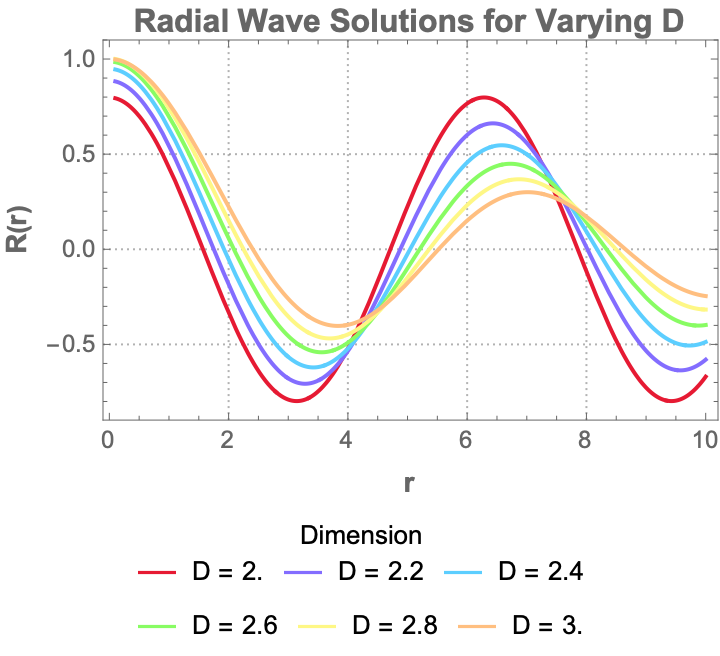
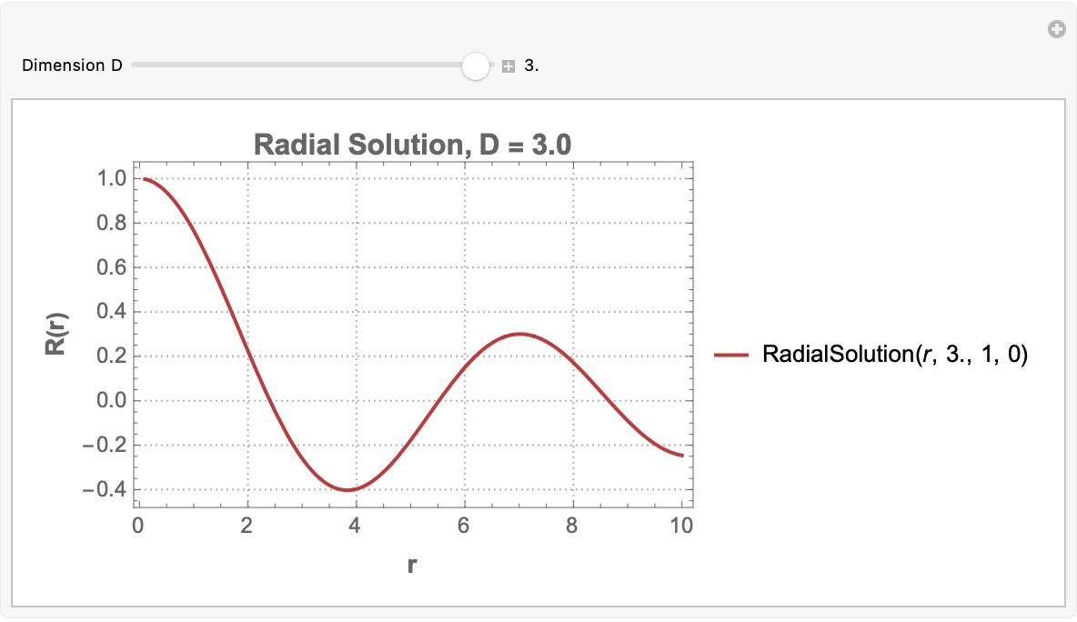
Some more wave and potential solutions in spaces of fractional dimension D between 2 and 3. We solve modified radial and vertical differential equations that describe how potentials or fields propagate differently when the spatial dimension is non-integer, such as D = 2.5. These solutions are expressed using Bessel functions and Gegenbauer polynomials, capturing radial, angular, and axial behaviors. The resulting plots illustrate how the wave structure, oscillations, and decay patterns evolve as D varies, offering discussions about photon propagation, gravity, or field behavior in non-Euclidean or fractal-like spaces.
ClearAll[radialWave];
radialWave[r_, d_, m_, k_] :=
  r^((3 - d)/2)  BesselJ[(d - 3)/2 + m, k  r];
Manipulate[
 Module[{colFrac, colStd},
  colFrac = ColorData["DarkRainbow"][Rescale[d, {2, 3}]];
  colStd = GrayLevel[0.4];
  Plot[{radialWave[r, d, m, k], radialWave[r, 3, m, k]}, {r, 0.1, 10},
    PlotTheme -> "Detailed", ImageSize -> 500, PlotRange -> {-1, 1},
   PlotStyle -> {{colFrac, Thick}, {colStd, Dashed, Thick}},
   Filling -> {1 -> Axis},
   FillingStyle -> Directive[colFrac, Opacity[0.2]], Frame -> True,
   FrameLabel -> (Style[#, 14, Bold] & /@ {"r", "R(r)"}),
   FrameTicksStyle -> Directive[FontSize -> 12],
   GridLines -> Automatic,
   GridLinesStyle -> Directive[LightGray, Dashed],
   PlotLegends ->
    Placed[LineLegend[{colFrac, colStd}, {Style["Fractional D", 12],
       Style["Standard D=3", 12]}, LegendMarkerSize -> 30], Above],
   PlotLabel ->
    Style[Row[{"Radial Wave: ", Style["D=", Bold],
       NumberForm[d, {2, 1}], ", m=", m, ", k=", k}], 16,
     Bold]]], {{d, 3, "Dimension (D)"}, 2, 3, 0.1,
  Appearance -> "Labeled"}, {{m, 0, "Azimuthal Order (m)"}, 0, 2, 1,
  Appearance -> "Labeled"}, {{k, 1, "Wave Number (k)"}, 0.1, 5, 0.1,
  Appearance -> "Labeled"}, ControlPlacement -> Left]
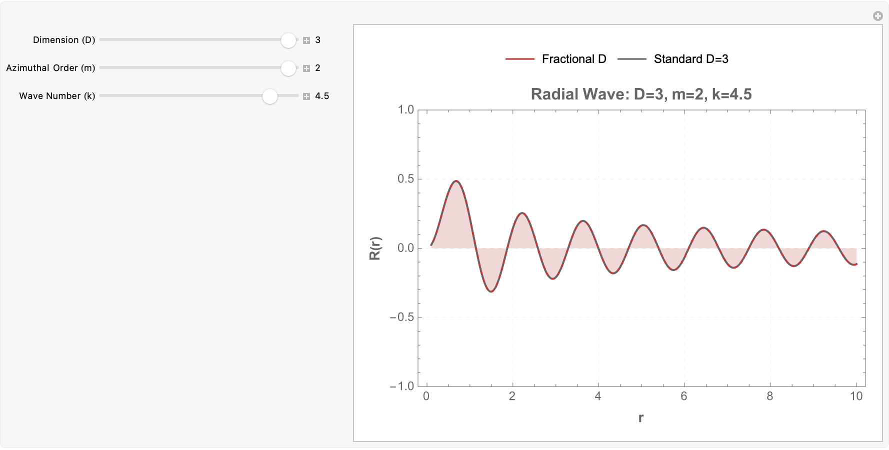
Now, before the rest of our article slips out of our hands like it was about to (if something happens to our article Simon Fischer we might simply create a new revised article with the attributes of the old), thus that is why I'm making a new reply. It probably has something to do with the length of the post. But that's not our fault. It's something to do with the shark who hosts these forum discussion boards, but no need to fear because I will be able to load them back up, and continue onward on our creation, of radial wave solutions in fractional-dimensional space versus standard three-dimensional space. We may need a new article for this; don't hesitate to tell them, there's a need to have more demonstrations, of the radial part of the wave equation using Bessel functions, because..the wave shape changes depending on the fractional dimension, the azimuthal mode number, and the wave number and in order to show the fractional dimension solution, and in order to more properly describe how waves would propagate differently in spaces that are not exactly three-dimensional, which is important for understanding not just photon propagation but also gravitational fields, in fractal-like geometries..so please bear with us, we've already described most of what we want to describe with regard to how fractional Laplacians can play a role in modifications to wave dispersion in slightly higher-level physics.


