In response to the question and some answers here: https://mathematica.stackexchange.com/q/291951
where we need to efficiently mowing a grass region using the least amount of time/fuel. The region can be concave and/or contain obstacles such as for example:

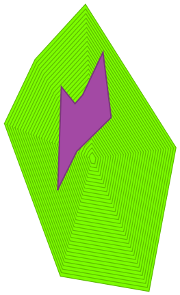
Here's my attempt, which is to take Vitaliy's method but try to mow along isolines of the region as much as possible. Essentially to try to 'spiral' inwards.

eq = x^2/2 - y^2 <= 1 && x^2 + y^2/7 > 1/2 && -3 < x < 3 && -3 < y < 3;
R = ImplicitRegion[eq, {x, y}];

reg = BoundaryDiscretizeRegion[R];

Attempt 1 (times out)

The idea is to discretize the region a certain distance from the boundary, then add 'bridge' edges across the isolines, where these bridges are weighted with a larger penalty. Then call FindShortestTour.

$bds = {};

reg2 = reg;
w = 0.1;

While[reg2 =!= EmptyRegion[2],
 (* remesh the curve to have nice sampling *)
 AppendTo[$bds, RegionBoundary@BoundaryDiscretizeRegion[
   ImplicitRegion[SignedRegionDistance[reg2][{x, y}] <= 0 && -3 < x < 3 && -3 < y < 3, {x, y}], MaxCellMeasure -> {1 -> w}]];
 reg2 = BoundaryDiscretizeRegion[RegionErosion[reg2, w]];
]

Length[crossedges = (Join @@ ((Join @@ MapThread[Function[{c1, c2},c1 \[UndirectedEdge] #& /@ c2[[1;;UpTo[1]]]],{#1, Nearest[#2, #1, {All, 1.25w}]}])& @@@ Partition[MeshCoordinates /@ $bds, 2, 1]))]

Output: 2377

Length[cycleedges = UndirectedEdge @@@ MeshPrimitives[UTJoin[$bds], 1][[All, 1]]]

Output: 2683

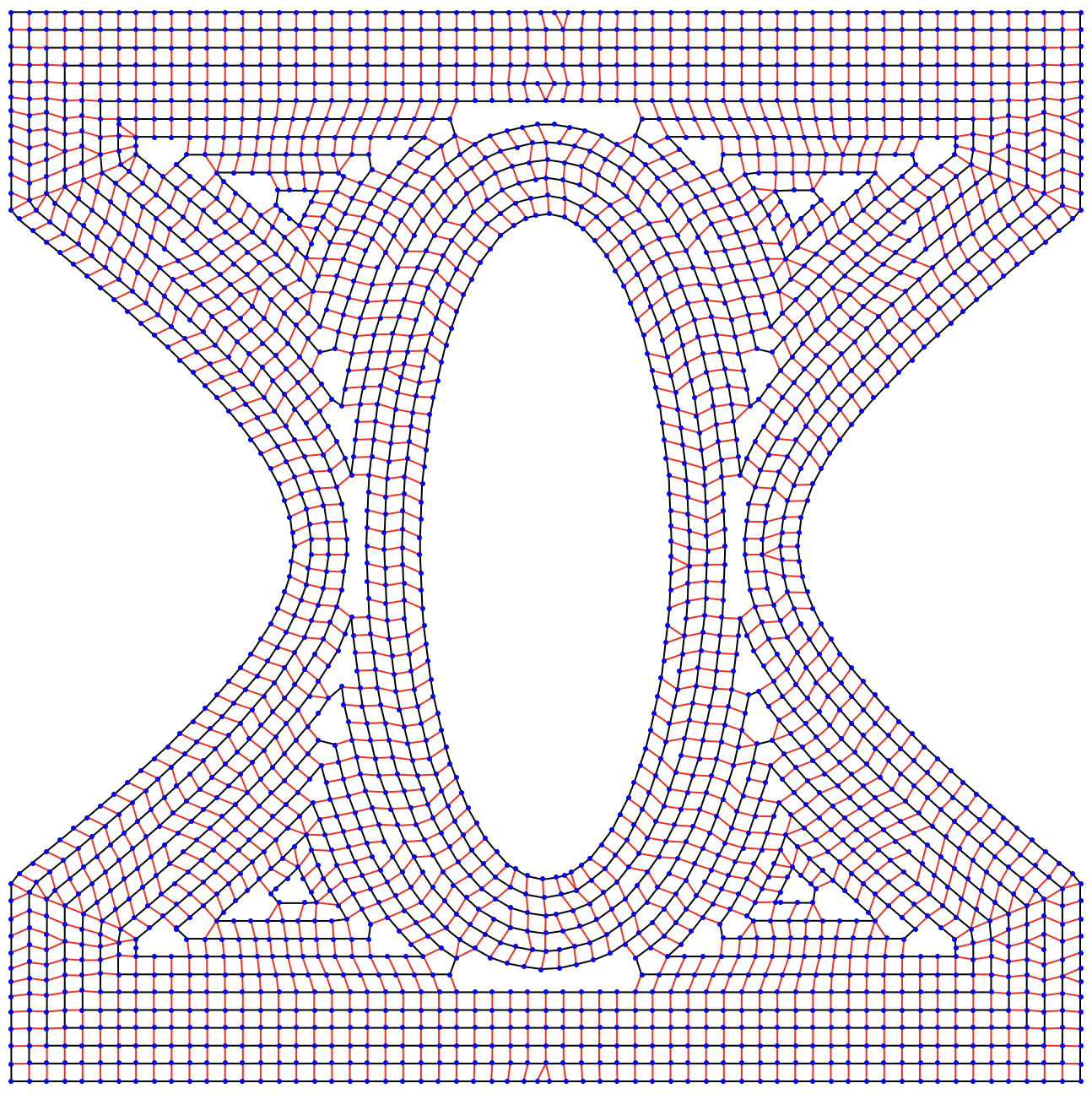
Here we want to travel along the black edges, and will sometimes bridge across the red edges:

Graphics[{
  Line[List @@@ cycleedges[[1 ;; -1]]],
  {Red, Line[List @@@ crossedges[[1 ;; -1 ;; 1]]]},
  {Blue, Point[MeshCoordinates[UTJoin[$bds]]]}
}]

Build the (weighted) graph:

g = Graph[
  MeshCoordinates[UTJoin[$bds]],
  Join[cycleedges, crossedges],
  EdgeWeight -> 
    Join[(# -> EuclideanDistance @@ #) & /@ 
      cycleedges, (# -> 100 EuclideanDistance @@ #) & /@ crossedges],
  VertexCoordinates -> MeshCoordinates[UTJoin[$bds]]
];

But FindShortestTour times out:

FindShortestTour[g]

$Aborted

Attempt 2

To work around this time out, we can pass a point cloud to FindShortestTour instead, lifting into 3D where each isoline will be in its own plane. Jumping 'up' in 3D will be the penalty for changing isolines.

Using $bds from above:

pts = Join @@ MapIndexed[Append[1.25 w (First[#2] - 1)] /@ #1 &, MeshCoordinates /@ $bds];

c = Nearest[pts, {-1000, 1000, 0}][[1]];

tour = FindShortestTour[pts, c, c]; // AbsoluteTiming

Output: {6.93906, Null}

path = pts[[tour[[2]], 1 ;; 2]];

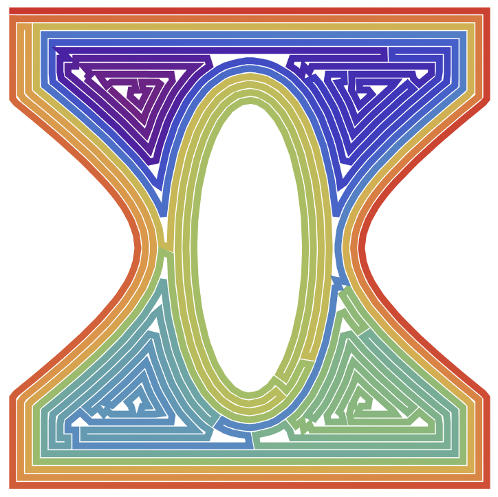
We can visualize the 'spiral' path with a color gradient:

colors = ColorData["Rainbow"] /@ Subdivide[1.0, 0.0, Length[path] - 1]];
Graphics[{AbsoluteThickness[5], Line[path, VertexColors -> colors}]

There's clearly still room for improvement, but it's still a start for sure.