Please tell me what is my mistake in implementing the calculation of the integral with a variable lower limit using the trapezoid method?
b[t_]:=t;(*a=1;*)
SigmaRhoBegin[rho_,phi_]=0;
(*Print["SigmaRhoBegin = ",SigmaRhoBegin[rho,phi]];*)
SigmaRhoPhiBegin[rho_,phi_]=0;
(*Print["SigmaRhoPhiBegin = ",SigmaRhoPhiBegin[rho,phi]];*)
(*delta=0;(*deltamin*)*)
(*delta=0.1*a;(*deltasr*)*)
(*delta=0.7*a;(*deltamax*)*)
delta=0.1;
(*bend=2*a;*)
(*L=bend+delta+0.1*a;(*Lmin*)*)
(*L=bend+delta+0.3*a;(*Lsr*)*)
(*L=(bend+delta+0.1*a)*5;(*Lmax*)*)
L=2.2;
varepsnom[rho_]=0.001;
F[rho_,phi_]=(lambda*Cos[phi]+rho/L)*Cos[phi]-Sqrt[1-(lambda*Cos[phi]+rho/L)^2]*Sin[phi];
lambda=delta/L;
varepsilon[rho_,phi_]=(varepsnom[rho]+1)*Sqrt[1+(lambda^2-2*lambda*F[rho,phi])/(1-(rho/L)^2)]-1;
nu=0.23;
EE=2*G*(1+nu);
SigmaPhiBegin[rho_,phi_]=EE*varepsilon[rho,phi]/G;
Print["SigmaPhiBegin = ",SigmaPhiBegin[rho,phi]];
(*Print["Min[oldp[rho,phi]] = ",NMinimize[SigmaPhiBegin[2(*rho*),phi],-Pi<=phi<=Pi,phi]];*)
Show[
Plot[(*{SigmaPhiBegin[1,phi],SigmaPhiBegin[1.2,phi],SigmaPhiBegin[1.4,phi],SigmaPhiBegin[1.6,phi],SigmaPhiBegin[1.8,phi],SigmaPhiBegin[2,phi]},*)SigmaPhiBegin[1.0,phi],{phi,-Pi,Pi},
AxesLabel->{"phi","Subscript[\[Sigma], \[Phi]\[Phi]]^*[rho,phi]"},
PlotRange->{{-Pi,Pi},{-0.8,0.7}},
GridLines->{Range[-3.4,3.4,0.2],Range[-0.8,0.7,0.05]},
PlotLegends->{"Subscript[\[Sigma], \[Phi]\[Phi]]^*[1.0,phi]","Subscript[\[Sigma], \[Phi]\[Phi]]^*[1.2,phi]","Subscript[\[Sigma], \[Phi]\[Phi]]^*[1.4,phi]","Subscript[\[Sigma], \[Phi]\[Phi]]^*[1.6,phi]","Subscript[\[Sigma], \[Phi]\[Phi]]^*[1.8,phi]","Subscript[\[Sigma], \[Phi]\[Phi]]^*[2.0,phi]"}
],
Graphics[{Arrow[{{-Pi,0},{Pi,0}}],Arrow[{{0,-0.8},{0,0.7}}]}]
]
{MAX,{max}}=Maximize[SigmaPhiBegin[1.0,phi],-Pi<=phi<=Pi,phi];
Print["Maximize[SigmaPhiPhiBegin[1.0,",max,"]] = ",MAX];
{MIN,{min}}=Minimize[SigmaPhiBegin[1.0,phi],-Pi<=phi<=Pi,phi];
Print["Minimize[SigmaPhiPhiBegin[1.0,",min,"]] = ",MIN];
(*--------------------------------------------------------------------------------------------------------------------------------*)
qbegin[rho_,phi_]=D[SigmaRhoPhiBegin[rho,phi],rho]+(D[SigmaPhiBegin[rho,phi],phi]+2*SigmaRhoPhiBegin[rho,phi])/rho;
q[t_,phi_]=qbegin[b[t],phi]*D[b[t],t];
(*Print["q[t,phi] = ",q[t,phi]];*)
pbegin[rho_,phi_]=D[SigmaRhoBegin[rho,phi],rho]+(D[SigmaRhoPhiBegin[rho,phi],phi]+SigmaRhoBegin[rho,phi]-SigmaPhiBegin[rho,phi])/rho;
p[t_,phi_]=-pbegin[b[t],phi]*D[b[t],t];
(*Print["p[t,phi] = ",p[t,phi]];*)
(*--------------------------------------------------------------------------------------------------------------------------------*)
(*--------------------------------------------------------------------------------------------------------------------------------*)
dotsigmarhophi[t_,phi_]=q[t,phi];
(*Print["dotsigmarhophi[t,phi] = ",dotsigmarhophi[t,phi]];*)
dotsigmarhorho[t_,phi_]=-p[t,phi];
(*Print["dotsigmarhorho[t,phi] = ",dotsigmarhorho[t,phi]];*)dotsigmaphiphi[t_,phi_]=D[dotsigmarhophi[t,phi],phi]+(t*D[dotsigmarhorho[t,phi],t]+dotsigmarhorho[t,phi]);
(*Print["dotsigmaphiphi[t,phi] = ",dotsigmaphiphi[t,phi]];*)
(*--------------------------------------------------------------------------------------------------------------------------------*)
(*------------------------------------------------------------------------------------------------------------------------------*)
Show[
Plot[{dotsigmarhophi[1,phi],dotsigmarhophi[1.2,phi],dotsigmarhophi[1.4,phi],dotsigmarhophi[1.6,phi],dotsigmarhophi[1.8,phi],dotsigmarhophi[2,phi]},{phi,-Pi,Pi},
AxesLabel->{"phi","Subscript[Overscript[\[Sigma], .], \[Rho]\[Phi]][t,phi]"},
PlotRange->{{-Pi,Pi},{-0.4,0.5}},
GridLines->{Range[-3.4,3.4,0.2],Range[-0.4,0.5,0.05]},
PlotLegends->{"Subscript[Overscript[\[Sigma], .], \[Rho]\[Phi]][1.0,phi]","Subscript[Overscript[\[Sigma], .], \[Rho]\[Phi]][1.2,phi]","Subscript[Overscript[\[Sigma], .], \[Rho]\[Phi]][1.4,phi]","Subscript[Overscript[\[Sigma], .], \[Rho]\[Phi]][1.6,phi]","Subscript[Overscript[\[Sigma], .], \[Rho]\[Phi]][1.8,phi]","Subscript[Overscript[\[Sigma], .], \[Rho]\[Phi]][2.0,phi]"}],
Graphics[{Arrow[{{-Pi,0},{Pi,0}}],Arrow[{{0,-0.4},{0,0.5}}]}]
]
Show[
Plot[{dotsigmarhorho[1,phi],dotsigmarhorho[1.2,phi],dotsigmarhorho[1.4,phi],dotsigmarhorho[1.6,phi],dotsigmarhorho[1.8,phi],dotsigmarhorho[2,phi]},{phi,-Pi,Pi},
AxesLabel->{"phi","Subscript[Overscript[\[Sigma], .], \[Rho]\[Rho]][t,phi]"},
PlotRange->{{-Pi,Pi},{-0.4,0.5}},
GridLines->{Range[-3.4,3.4,0.2],Range[-0.4,0.5,0.05]},
PlotLegends->{"Subscript[Overscript[\[Sigma], .], \[Rho]\[Rho]][1.0,phi]","Subscript[Overscript[\[Sigma], .], \[Rho]\[Rho]][1.2,phi]","Subscript[Overscript[\[Sigma], .], \[Rho]\[Rho]][1.4,phi]","Subscript[Overscript[\[Sigma], .], \[Rho]\[Rho]][1.6,phi]","Subscript[Overscript[\[Sigma], .], \[Rho]\[Rho]][1.8,phi]","Subscript[Overscript[\[Sigma], .], \[Rho]\[Rho]][2.0,phi]"}],
Graphics[{Arrow[{{-Pi,0},{Pi,0}}],Arrow[{{0,-0.4},{0,0.5}}]}]
]
Show[
Plot[{dotsigmaphiphi[1,phi],dotsigmaphiphi[1.2,phi],dotsigmaphiphi[1.4,phi],dotsigmaphiphi[1.6,phi],dotsigmaphiphi[1.8,phi],dotsigmaphiphi[2,phi]},{phi,-Pi,Pi},
AxesLabel->{"phi","Subscript[Overscript[\[Sigma], .], \[Phi]\[Phi]][t,phi]"},
PlotRange->{{-Pi,Pi},{-3,5}},
GridLines->{Range[-3.4,3.4,0.2],Range[-3,5,0.5]},
PlotLegends->{"Subscript[Overscript[\[Sigma], .], \[Phi]\[Phi]][1.0,phi]","Subscript[Overscript[\[Sigma], .], \[Phi]\[Phi]][1.2,phi]","Subscript[Overscript[\[Sigma], .], \[Phi]\[Phi]][1.4,phi]","Subscript[Overscript[\[Sigma], .], \[Phi]\[Phi]][1.6,phi]","Subscript[Overscript[\[Sigma], .], \[Phi]\[Phi]][1.8,phi]","Subscript[Overscript[\[Sigma], .], \[Phi]\[Phi]][2.0,phi]"}],
Graphics[{Arrow[{{-Pi,0},{Pi,0}}],Arrow[{{0,-3},{0,5}}]}]
]
(*------------------------------------------------------------------------------------------------------------------------------*)
(*------------------------------------------------------------------------------------------------------------------------------*)
fitWithAdaptiveOrder[T_,f_]:=
Module[{func,m,data,model,vars,fit,approx,epsilon,cleanFit},
epsilon=0.01;
func[t_,phi_]:=f[t,phi];
m=3;
While[True,
data=Table[{phi,func[T,phi]},{phi,-Pi,Pi,Pi/m}];
model=a0+Sum[ak[k]*Cos[k*phi]+bk[k]*Sin[k*phi],{k,1,Ceiling[m/2]-1}];
vars=Join[{a0},Flatten[Table[{ak[k],bk[k]},{k,1,Ceiling[m/2]-1}]]];
fit=FindFit[data,model,vars,phi];
(*cleanFit=fit/.Rule[coeff_,val_]:>Rule[coeff,If[Abs[val]<10^(-10),0,val]];
approx=model/.cleanFit;*)
approx=model/.fit;
(*If[func[T,phi]!=0,*)
If[Max[Abs[Table[Abs[(approx-func[T,phi])/func[T,phi]]/. phi->x,{x,-Pi,Pi,Pi/m}]]]<epsilon,Break[]];(*,
If[Max[Abs[Table[Abs[approx-func[T,phi]/.{ phi->x}],{x,-Pi,Pi,Pi/m}]]]<epsilon,Break[]];(*Если Delta=0*)
];*)
m=m+1;
];
approx];
(*------------------------------------------------------------------------------------------------------------------------------*)
(*------------------------------------------------------------------------------------------------------------------------------*)
approxFunction1[t_,theta_]:=fitWithAdaptiveOrder[t,q]/.{phi->theta};
Time=2.0;Phi=Pi/2;
Print["approxFunction1[",Time,",pHi] = ",approxFunction1[Time,pHi]];
Print["approxFunction1[",Time,",",Phi,"] = ",approxFunction1[Time,Phi]];
Print["q[",Time,",",Phi,"] = ",approxFunction1[Time,Phi]];
(*------------------------------------------------------------------------------------------------------------------------------*)
(*------------------------------------------------------------------------------------------------------------------------------*)
timebeginRP=AbsoluteTime[];
uRP=0.4;
flagI1nRP=True;
epsilonRP=0.0002;
delta2nRP=100.;
NNRP=100;
I1nRP=Table[-100.,{i,1,NNRP}];I2nRP=Table[-100.,{i,1,NNRP}];
X1nRP=Table[-100.,{i,1,NNRP}];X2nRP=Table[-100.,{i,1,NNRP}];
Y1nRP=Table[-100.,{i,1,NNRP}];Y2nRP=Table[-100.,{i,1,NNRP}];
rho0RP=1;
rhofRP=2;
t0RP=1;
tfRP=2;
While[delta2nRP>epsilonRP,
delta2nRP=-1.;
uRP=uRP/2;
I1nRP=I2nRP;
I2nRP=Table[-100.,{i,1,NNRP}];
X1nRP=X2nRP;
Y1nRP=Y2nRP;
Do[(*For[v=1,v<=2,v=v+1,*)
If[v==2||(v==1&&flagI1nRP==True),
flagI1nRP=False;
flagRP=v==1;
dtRP=uRP/v;(*integration step*)
(*number of time segments. (+1) to take into account the tfRP time point, which we will add artificially*)
iendRP=Round[(tfRP-t0RP)/dtRP]+1;
fouriendRP=4*iendRP+1;(*number of grid division angles. (+1) to include Pi*)
spisoksigmaPSKRP=Table[Table[Table[{0.,0.,0.},{j,1,fouriendRP}],{s,1,iendRP}],{i,1,iendRP}];
Do[(*For[i=1,i<=iendRP,i=i+1,*)(*RHO radius cycle*)
tempRP=t0RP+(i-1)*dtRP;(*current time layer*)
RhoRP=rho0RP+(i-1)*dtRP;(*current radius*)
(*at each new time layer-radius we initialize the initial value of the function*)
sigmanewValRP=SigmaRhoPhiBegin[tempRP,phi];
Do[(*For[t=tempRP,t<=tfRP-dtRP,t=t+dtRP,*)(*Time cycle T*)
sigmanewValRP=sigmanewValRP+dtRP*(fitWithAdaptiveOrder[t,dotsigmarhophi]+fitWithAdaptiveOrder[t+dtRP,dotsigmarhophi])/2/.{phi->theta};
(*Print["sigmanewValRP = ",sigmanewValRP];*)
timeRP=Round[(t-t0RP)/dtRP]+1;
Do[(*For[j=1,j<=fouriendRP,j=j+1,*)(*Cycle by angle PHI*)
thetaRP=-(Pi+(2*Pi)/(4*iendRP))+(2*Pi*j)/(4*iendRP);(*-Pi<=phi<=Pi*)
resRP=Evaluate[sigmanewValRP/.{theta->thetaRP}];
If[v==1,
spisoksigmaPSKRP[[i]][[timeRP]][[j]]={RhoRP,thetaRP,resRP};,(*filled only on the first iteration, then blocked*)
spisoksigmaPSKRP[[i]][[timeRP+1]][[j]]={RhoRP,thetaRP,resRP};(*filled in at each iteration*)
];
If[t==tfRP-dtRP&&resRP>I1nRP[[i]]&&flagRP==True,(*we are looking for the maximum value of the integral on the penultimate time layer*)
I1nRP[[i]]=resRP;
X1nRP[[i]]=RhoRP;
Y1nRP[[i]]=thetaRP;
];
If[t==tfRP-dtRP&&resRP>I2nRP[[i]]&&flagRP==False,
I2nRP[[i]]=resRP;
X2nRP[[i]]=RhoRP;
Y2nRP[[i]]=thetaRP;
];
(*Angle (theta(phi)) from -Pi to Pi*)
,{j,1,fouriendRP,1}];(*];*)
(*Cycle to the penultimate time layer, since the trapezoid method uses the current and next steps*)
,{t,tempRP,tfRP-dtRP,dtRP}];(*];*)
(*Rho radii from 1.0 to 1.9, since we don’t add anything to the first one, since (i-1)*dt*)
,{i,1,iendRP,1}];(*];*)
];
(*we calculate the integral with step h, then with step h/2 and compare the results using the Runge method, we calculate both integrals only at the 1st iteration, and then flag=False*)
,{v,1,2,1}];(*];*)
Do[(*For[z=1,z<=NNRP/2,z=z+1,*)
errorRP=Abs[I2nRP[[2*z-1]]-I1nRP[[z]]]/3;
If[delta2nRP<errorRP,
delta2nRP=errorRP;
iiRP=z;
];
,{z,1,NNRP/2,1}];(*];*)
Print["------------------------------------------------------------------------------------------------------------------------"];
Print["ii = ",iiRP,", u = ",uRP];
Print["I1n[",X1nRP[[iiRP]],",",Y1nRP[[iiRP]],"] = ",I1nRP[[iiRP]],", I2n[",X2nRP[[2*iiRP-1]],",",Y2nRP[[2*iiRP-1]],"] = ",I2nRP[[2*iiRP-1]],", delta2n = ",delta2nRP];
];
timeendRP=AbsoluteTime[];
Print["Time: ",(timeendRP-timebeginRP)/60];
Do[(*For[i=1,i<=iendRP,i=i+1,*)
RhoRP=rho0RP+(i-1)*dtRP;
Do[(*For[Time=t0RP,Time<=tfRP,Time=Time+dtRP,*)
newtimeRP=Round[(Time-t0RP)/dtRP]+1;
If[i==newtimeRP(*&&RhoRP>1.*),
Do[
thetaRP=-(Pi+(2*Pi)/(4*iendRP))+(2*Pi*j)/(4*iendRP);
resRP=SigmaRhoPhiBegin[RhoRP,thetaRP];
spisoksigmaPSKRP[[i]][[newtimeRP]][[j]]={RhoRP,thetaRP,resRP};
(*If[RhoRP>1.0,
XRP=RhoRP*Cos[thetaRP];
YRP=RhoRP*Sin[thetaRP];
spisoksigmaDSKRP[[i]][[newtimeRP]][[j]]={XRP,YRP,resRP};
];*)
,{j,1,fouriendRP,1}];
];
,{Time,t0RP,tfRP,dtRP}];(*];*)
,{i,1,iendRP,1}];(*];*)
(*------------------------------------------------------------------------------------------------------------------------------*)
(*------------------------------------------------------------------------------------------------------------------------------*)
timebeginRR=AbsoluteTime[];
uRR=0.4;
flagI1nRR=True;
epsilonRR=0.0001;
delta2nRR=100.;
NNRR=100;
I1nRR=Table[-100.,{i,1,NNRR}];I2nRR=Table[-100.,{i,1,NNRR}];
X1nRR=Table[-100.,{i,1,NNRR}];X2nRR=Table[-100.,{i,1,NNRR}];
Y1nRR=Table[-100.,{i,1,NNRR}];Y2nRR=Table[-100.,{i,1,NNRR}];
rho0RR=1;
rhofRR=2;
t0RR=1;
tfRR=2;
While[delta2nRR>epsilonRR,
delta2nRR=-1.;
uRR=uRR/2;
I1nRR=I2nRR;
I2nRR=Table[-100.,{i,1,NNRR}];
X1nRR=X2nRR;
Y1nRR=Y2nRR;
Do[(*For[v=1,v<=2,v=v+1,*)
If[v==2||(v==1&&flagI1nRR==True),
flagI1nRR=False;
flagRR=v==1;
dtRR=uRR/v;
iendRR=Round[(tfRR-t0RR)/dtRR]+1;
fouriendRR=4*iendRR+1;
(*spisoksigmaDSKRR=Table[Table[Table[{0.,0.,0.},{j,1,fouriendRR}],{s,1,iendRR}],{i,1,iendRR}];*)
spisoksigmaPSKRR=Table[Table[Table[{0.,0.,0.},{j,1,fouriendRR}],{s,1,iendRR}],{i,1,iendRR}];
Do[(*For[i=1,i<=iendRR,i=i+1,*)
tempRR=t0RR+(i-1)*dtRR;
RhoRR=rho0RR+(i-1)*dtRR;
sigmanewValRR=SigmaRhoBegin[tempRR,phi];
Do[(*For[t=tempRR,t<=tfRR-dtRR,t=t+dtRR,*)
sigmanewValRR=sigmanewValRR+dtRR*(fitWithAdaptiveOrder[t,dotsigmarhorho]+fitWithAdaptiveOrder[t+dtRR,dotsigmarhorho])/2/.{phi->theta};
timeRR=Round[(t-t0RR)/dtRR];
Do[(*For[j=1,j<=fouriendRR,j=j+1,*)
thetaRR=Evaluate[-(Pi+(2*Pi)/(4*iendRR))+(2*Pi*j)/(4*iendRR)];(*-Pi<=Phi<=Pi*)
resRR=Evaluate[sigmanewValRR/.{theta->thetaRR}];
If[v==1,
spisoksigmaPSKRR[[i]][[timeRR+1]][[j]]={RhoRR,thetaRR,resRR};,
spisoksigmaPSKRR[[i]][[timeRR+2]][[j]]={RhoRR,thetaRR,resRR};
];
If[t==tfRR-dtRR&&resRR>I1nRR[[i]]&&flagRR==True,
I1nRR[[i]]=resRR;
X1nRR[[i]]=RhoRR;
Y1nRR[[i]]=thetaRR;
];
If[t==tfRR-dtRR&&resRR>I2nRR[[i]]&&flagRR==False,
I2nRR[[i]]=resRR;
X2nRR[[i]]=RhoRR;
Y2nRR[[i]]=thetaRR;
];
,{j,1,fouriendRR,1}];(*];*)
,{t,tempRR,tfRR-dtRR,dtRR}];(*];*)
,{i,1,iendRR,1}];(*];*)
];
,{v,1,2,1}];(*];*)
Do[(*For[z=1,z<=NNRR/2,z=z+1,*)
errorRR=Abs[I2nRR[[2*z-1]]-I1nRR[[z]]]/3;
If[delta2nRR<errorRR,
delta2nRR=errorRR;
iiRR=z;
];
,{z,1,NNRR/2,1}];(*];*)
Print["------------------------------------------------------------------------------------------------------------------------"];
Print["ii = ",iiRR,", u = ",uRR];
Print["I1n[",X1nRR[[iiRR]],",",Y1nRR[[iiRR]],"] = ",I1nRR[[iiRR]],", I2n[",X2nRR[[2*iiRR-1]],",",Y2nRR[[2*iiRR-1]],"] = ",I2nRR[[2*iiRR-1]],", delta2n = ",delta2nRR];
];
timeendRR=AbsoluteTime[];
Print["Time: ",(timeendRR-timebeginRR)/60];
Do[(*For[i=1,i<=iendRR,i=i+1,*)
RhoRR=rho0RR+(i-1)*dtRR;
Do[(*For[Time=t0RR,Time<=tfRR,Time=Time+dtRR,*)
newtimeRR=Round[(Time-t0RR)/dtRR]+1;
If[i==newtimeRR(*&&RhoRR>1.*),
Do[
thetaRR=Evaluate[-(Pi+(2*Pi)/(4*iendRR))+(2*Pi*j)/(4*iendRR)];
resRR=SigmaRhoBegin[RhoRR,thetaRR];
spisoksigmaPSKRR[[i]][[newtimeRR]][[j]]={RhoRR,thetaRR,resRR};
(*If[RhoRR>1.,
XRR=RhoRR*Cos[thetaRR];
YRR=RhoRR*Sin[thetaRR];
spisoksigmaDSKRR[[i]][[newtimeRR]][[j]]={XRR,YRR,resRR};
];*)
,{j,1,fouriendRR,1}];
];
,{Time,t0RR,tfRR,dtRR}];(*];*)
,{i,1,iendRR,1}];(*];*)
(*------------------------------------------------------------------------------------------------------------------------------*)
(*--------------------------------------------------------------------------------------------------------------------------------*)
tableRP={};
For[j=1,j<=fouriendRP,j=j+1,
If[spisoksigmaPSKRP[[1]][[iendRP]][[j]]!={0.,0.,0.},
tableRP=Append[tableRP,spisoksigmaPSKRP[[1]][[iendRP]][[j]]];
];
];
(*--------------------------------------------------------------------------------------------------------------------------------*)
(*--------------------------------------------------------------------------------------------------------------------------------*)
tableRR={};
For[j=1,j<=fouriendRR,j=j+1,
If[spisoksigmaPSKRR[[1]][[iendRR]][[j]]!={0.,0.,0.},
tableRR=Append[tableRR,spisoksigmaPSKRR[[1]][[iendRR]][[j]]];
];
];
(*--------------------------------------------------------------------------------------------------------------------------------*)
(*--------------------------------------------------------------------------------------------------------------------------------*)
ListLinePlot[
{tableRR,tableRP(*,tablePP[iendPP]*)}/. {a_,b_,c_}:>{b,c},
PlotStyle->Automatic,
PlotRange->{{-Pi,Pi},{-0.2,0.2}},(*{{-Pi,Pi},All},*)
AxesLabel->{"\[Phi]","\[Sigma]"},
ImageSize->Large,
GridLines->{Range[-3.2,3.2,0.2],Range[-0.2,0.2,0.02]}
]
(*--------------------------------------------------------------------------------------------------------------------------------*)
Below I attach 2 graphs. The first one is what should be obtained, the second one is what I get. 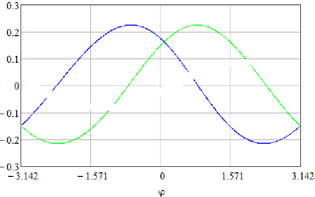
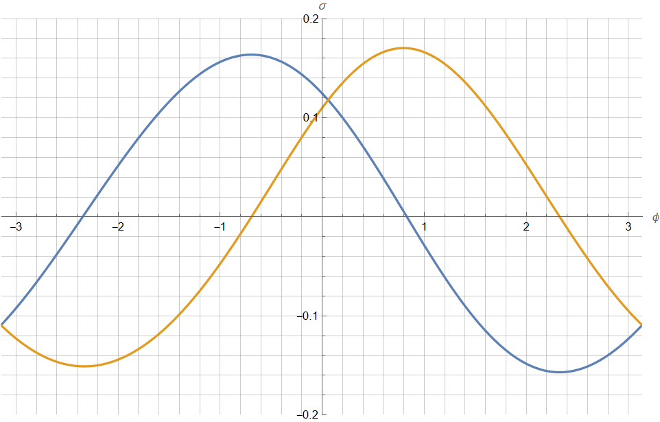
Note: The problem is that the graphs look the same, but the resulting vertical stress values are different.
This is my first time asking a question on this forum. When I click "Reply" for some reason nothing happens, so I'm answering you by editing the original post.
Eric, I wrote a program for a general case. Now I am considering a specific model. For which the input data is as follows. - - - - - - - - - - - - - - - - - - - - - - - - - - - - - - - - - - - - - - - - - - - - - - - - - - - - - - - - - - - - - - - - - - - - - - - - - I am considering the problem of body growth. b[t]=t is the growth function. It is the outer radius, t is time. The radius and time are sort of synchronized. The first part of the code is simply formulas rewritten into code. The integration itself begins with:
uRP=0.4;
flagI1nRP=True;
epsilonRP=0.0001;
delta2nRP=100.;
NNRP=100;
...
For the shear stress RR the integration function is similar.
The lower integration limit is "t", the upper one is "b(t)", for the model under consideration 1<=t<=2.


