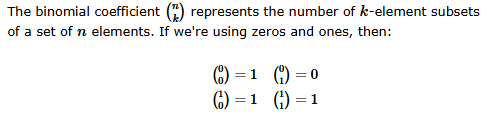
Part 2: https://community.wolfram.com/groups/-/m/t/3546261

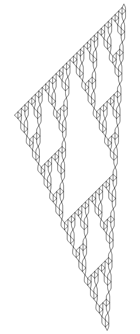
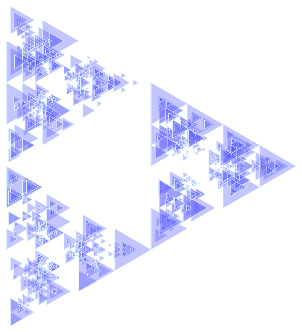
Constructing the Sierpinski triangle

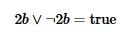
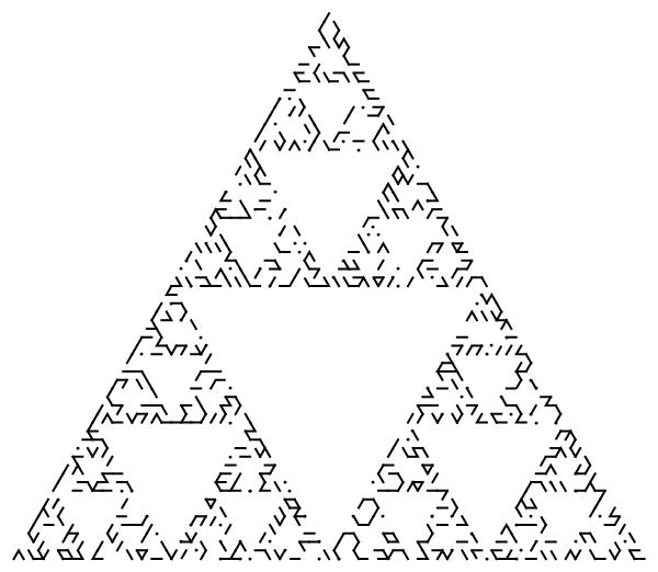
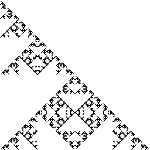
Throughout my years playing around with fractals, the Sierpinski triangle has been a consistent staple. The triangle is named after Wacław Sierpiński and as fractals are wont the pattern appears in many places, so there are many different ways of constructing the triangle on a computer.

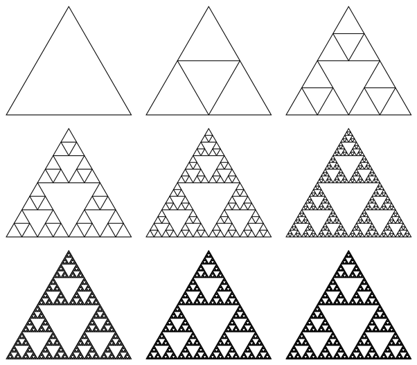
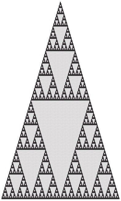
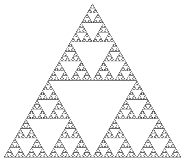
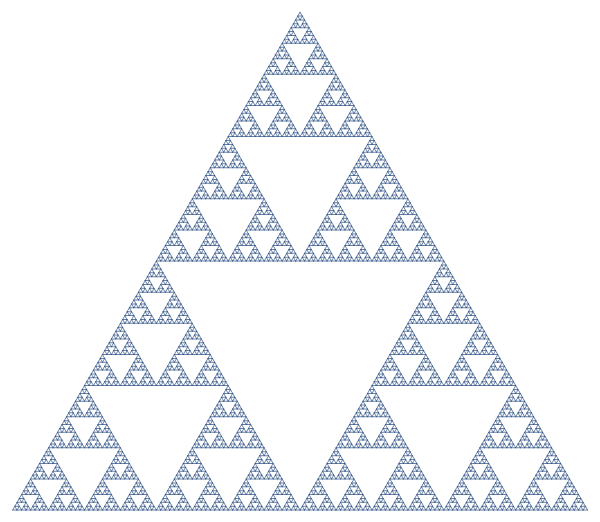
All of the methods are fundamentally iterative. The most obvious method is probably the triangle-in-triangle approach. We start with one triangle, and at every step we replace each triangle with 3 subtriangles:

axiom = Polygon[{{0, 0}, {1, Sqrt[3]}/2, {1, 0}}];

next[prev_] := prev /. Polygon[{p1_, p2_, p3_}] :> {
     Polygon[{p1, (p1 + p2)/2, (p1 + p3)/2}],
     Polygon[{p2, (p2 + p3)/2, (p1 + p2)/2}],
     Polygon[{p3, (p1 + p3)/2, (p2 + p3)/2}]};

draw[n_] := Graphics[{EdgeForm[Black],
    Nest[next, N@axiom, n]}];

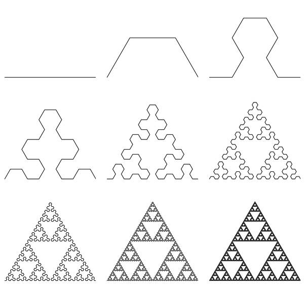
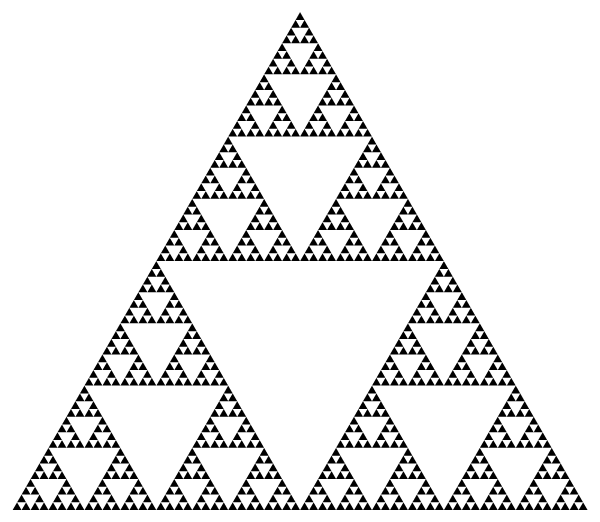
This triangle-in-triangle method strikes me as a disguised Lindenmayer system. L-systems are iterative symbol-based replacement mechanisms. There are a variety of more explicit L-system constructions for the triangle, such as the 'arrowhead' L-system (also see my L-systems program):

axiom = {A};
rules = {A -> {B, R, A, R, B}, B -> {A, L, B, L, A}};
conversions = {A -> forward, B -> forward, L -> left, R -> right};

(* state transformations *)
forward[{z_, a_}] := {z + E^(I a), a};
left[{z_, a_}] := {z, a + 2 Pi/6};
right[{z_, a_}] := {z, a - 2 Pi/6};

draw[n_] := Module[{program, zs},
  program = Flatten[Nest[# /. rules &, axiom, n]] /. conversions;
  zs = First /@ ComposeList[program, N@{0, 0}];
  Graphics[Line[{Re[#], Im[#]} & /@ First /@ Split[zs]]]];

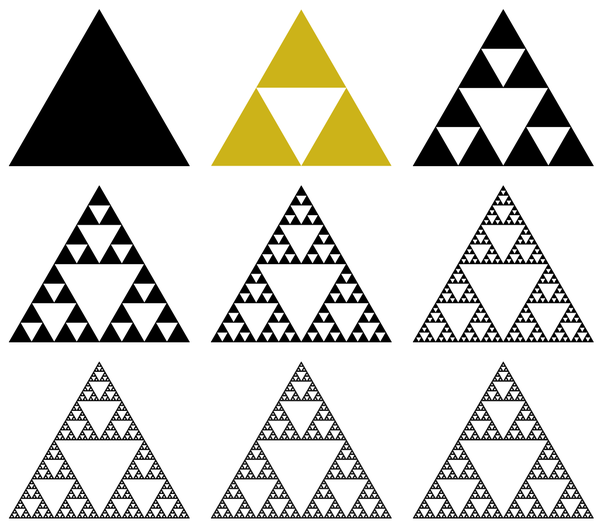
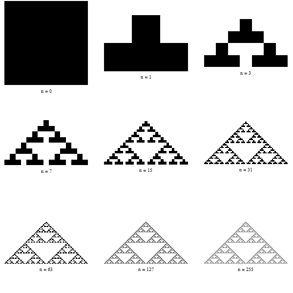
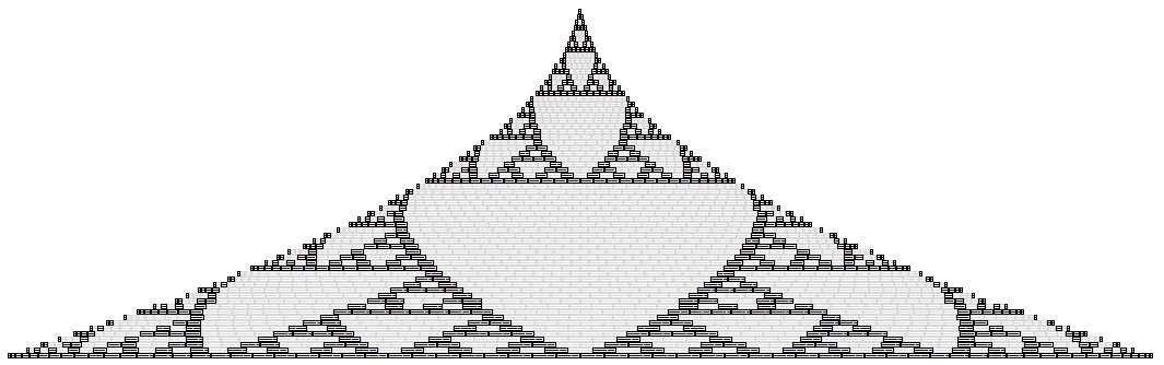
There's the cellular automata approach, where the 'world' is a single array of bits and at each "instant" we alter a bit based on the state of it and its neighbors. If we plot the evolution of Rule 22 (and others), we get these patterns:

draw[n_] := ArrayPlot[CellularAutomaton[22, {{1}, 0}, n]];

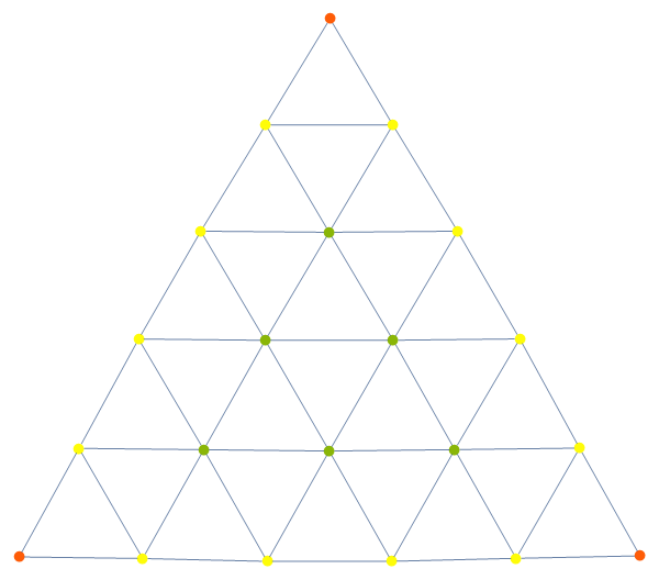
There are bound to be many elementary number-theoretic constructions of the Sierpinski triangle given that it looks like a percolation pattern (as in the cellular automata above). The Wikipedia article mentions that it appears in Pascal's Triangle when differentiating between even and odd numbers. Sure enough:

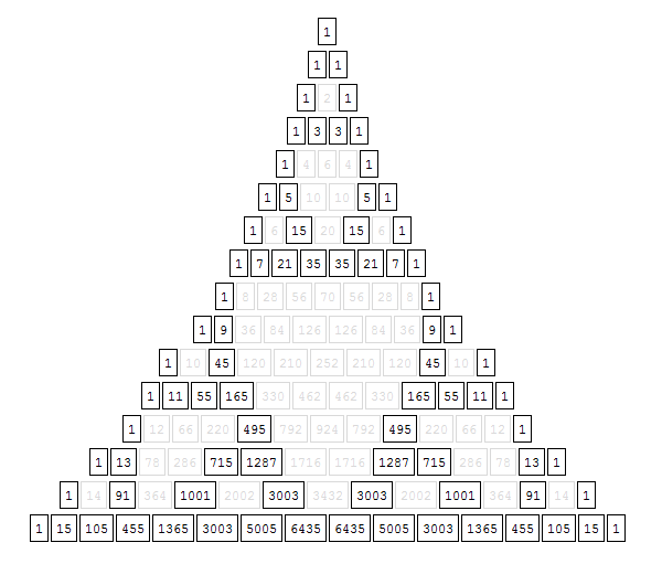
draw[n_] := Module[{t},
    t = Table[Binomial[m, k], {m, 0, n}, {k, 0, m}];

    Column[Row[#, " "] & /@ t, Center] /. {
        x_?EvenQ :> Style[Framed[x], LightGray],
        x_?OddQ :> Framed[x]}];

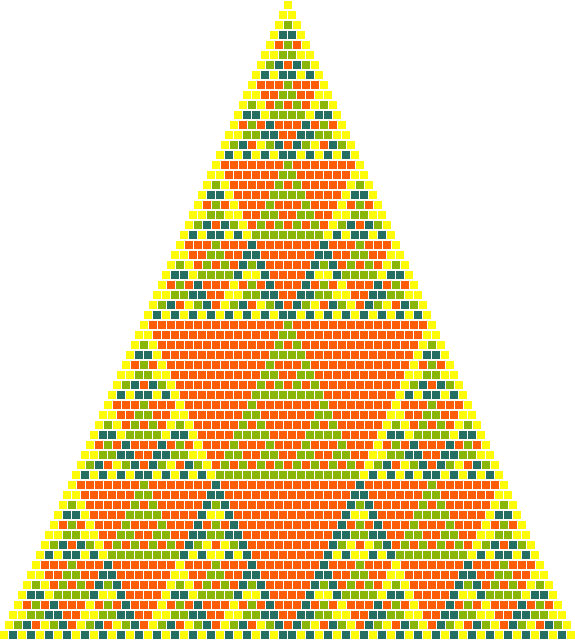
If we look at these Pascal forms and reverse engineer the parity rules, we get Rule 22. Though it might depend on what exactly you're reverse engineering. We can generalize from even/odd to other moduli:

Pascal's triangle mod 4:

Pascal's triangle x≡2 (mod 4):

draw[n_] := Module[{t},
   t = Table[Mod[Binomial[m, k], 4], {m, 0, n}, {k, 0, m}];

   Column[Row[#, " "] & /@ t, Center] /. x_?NumberQ :>
     Style[Framed["  ", FrameStyle -> None],
      Background -> ColorData[3][2 + x]]];

The Wikipedia article for Pascal's triangle mentions that we can construct a 'Pascal matrix' using the matrix exponential:

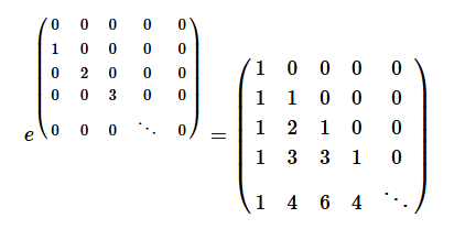
"Ah, that makes sense." You say. Indeed, but what's cool is that we then have a pedantic way of specifying the Sierpinski triangle:

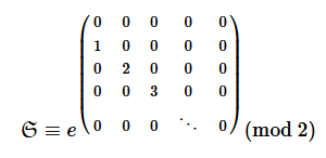
This equation is in what's called "straight ballin'" form, and it gives us a fancy way of producing the triangle:

draw[n_] := ArrayPlot[Mod[MatrixExp[DiagonalMatrix[Range[n], -1]], 2]];

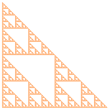
Heawt deaowg /drawl. It's not very performant though. The following is faster and arguably more elegant:

draw[n_] := ArrayPlot[Mod[Array[Binomial, {n, n}, 0], 2]];

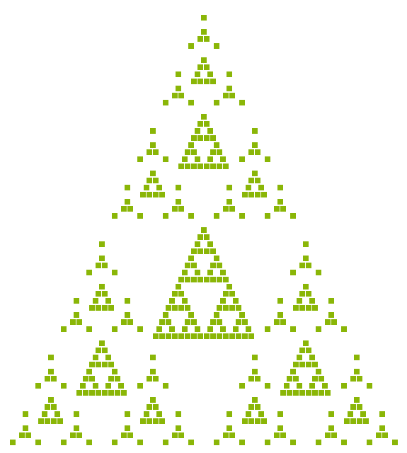
Along these lines, it shouldn't be surprising that the Sierpinski pattern appears in other combinatorial expressions, such as the Stirling numbers:

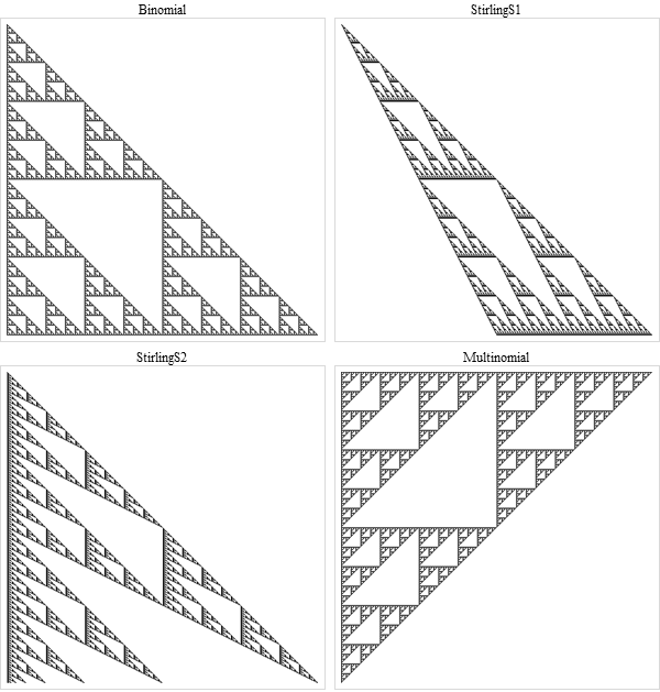
draw[n_] := Grid[Partition[#, 2]] &@
   Table[ArrayPlot[Mod[Array[f, {n, n}], 2],
     PlotLabel -> f, FrameStyle -> LightGray],
    {f, {Binomial, StirlingS1, StirlingS2, Multinomial}}];

If we treat the rows produced by these combinatorial functions as arrays of bits, what sequence of numbers do the bits represent? There's a variety of ways to interpret this question, but here's one assortment:

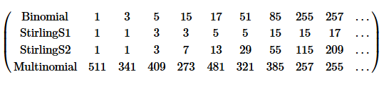
draw[n_] := With[{dropZeros = # /. {x__, 0 ..} :> {x} &},
   MatrixForm[Table[Flatten[
      {f, FromDigits[dropZeros[#], 2] & /@ Mod[Array[f, {n, n}, 0], 2], "\[Ellipsis]"}],
     {f, {Binomial, StirlingS1, StirlingS2, Multinomial}}]]];

The first, second, and fourth sequences are versions of each other, tautologically described in OEIS as A001317. The sequence for the Stirling numbers of the second kind doesn't seem to have any fame, but if you shift its bits around you can find A099901 and A099902.

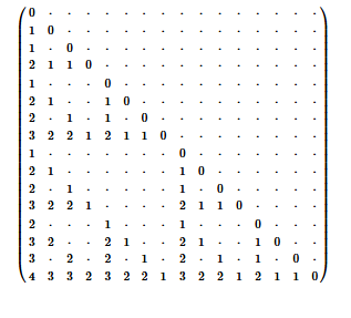
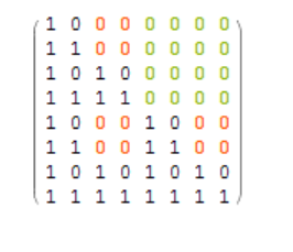
The Wikipedia article for the Sierpinski triangle mentions its appearance in logic tables such as this one. If you stare blankly at that image long enough you'll notice it's a set-inclusion table. Take the subsets of a set and pair them against each other under set-inclusion (is subset A a subset of subset B?) and you will get that table.

Personally that's a more interesting interpretation than the binary logic one, though the apparent distinction between these subjects is likely just a matter of perspective. Another set-related Sierpinski pattern I found is set disjunction (when sets have no common elements):

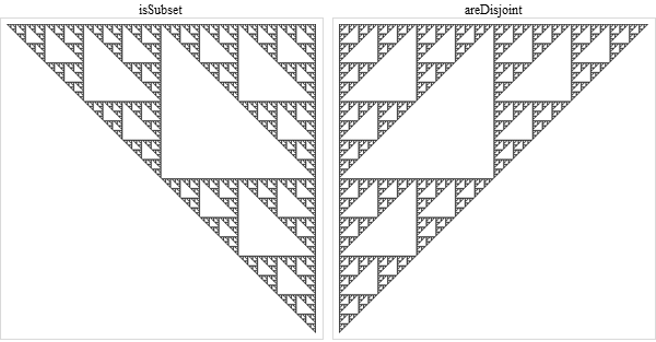
isSubset[a_, b_] := Union[a, b] == b;
areDisjoint[a_, b_] := Intersection[a, b] == {};

subs[0] = {{}};
subs[n_] := Module[{s = subs[n - 1]},
   Join[s, Append[#, n] & /@ s]];

draw[n_] := Grid[List[Table[
     ArrayPlot[Boole[Outer[f, subs[n], subs[n], 1]],
      PlotLabel -> f, FrameStyle -> LightGray],
     {f, {isSubset, areDisjoint}}]]]

One thing I noticed is that these set patterns depend on the order in which you place the subsets. It has to be the same order that you would get if you were constructing the subsets iteratively. I also wasn't able to find a straightforward ranking function that would order the sets into this iterative sequence. Mathematica's Combinatorica package refers to it as the binary ordering. I think I'm starting to understand what Gandalf meant when he said

"The Sierpinski triangle cannot-be wrought without heed to the creeping tendrils of recursion. Even the binomial coefficient has factorials which are recursively defined."

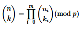
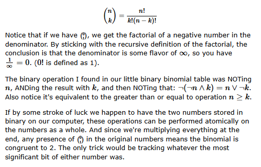
MathWorld mentions a broader context for why binary logic can be used in the construction of the Sierpinski triangle. Namely the Lucas correspondence theorem which states that given two numbers written in a prime base,

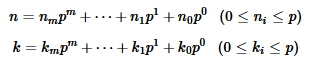
We can get their binomial coefficient modulo that prime by performing binomial coefficients digit-wise and multiplying the results.

TraditionalForm[Grid[Outer[
    HoldForm[Binomial[##]] == Binomial[##] &,
  {0, 1}, {0, 1}]]]

The factorial definition is interesting in this case.

binaryBinomial[a_, b_] := Module[{bits},
   bits = IntegerDigits[{a, b}, 2];
   bits = PadLeft[#, Max[Length /@ bits]] & /@ bits;

   Boole[FreeQ[Transpose[bits], {0, 1}]]];

draw[n_] := MatrixPlot[
   Array[binaryBinomial, {2^n, 2^n}, 0],
   Frame -> None];

There's a lot of related patterns:

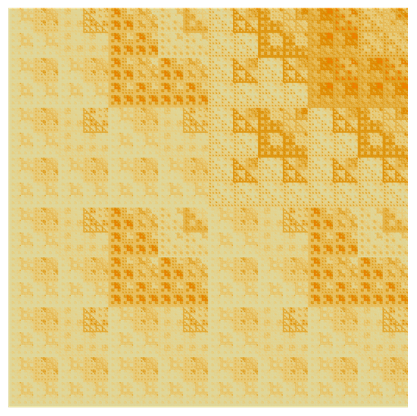
binaryWhoKnows[a_, b_] :=
  DigitCount[BitOr[a, BitNot[b]], 3, 1];

draw[n_] := MatrixPlot[
   Array[binaryWhoKnows, {2^n, 2^n}, 0],
   Frame -> False];

And look what I found!

If we're looking for a one- or two-liner that's one- or two-linear in languages beside Mathematica, we'd have trouble doing better than the chaos game algorithm, which goes like this:

1 start at any point. call it p
2 pick one of the three vertices at random
3 find the point halfway between p and that vertex
4 call that point p and draw it
5 goto 2

vertices = {{0, 0}, {1, Sqrt[3]}/2, {1, 0}};

draw[numPoints_] := Graphics[{
    PointSize[0], Opacity[.1],
    Point[FoldList[(#1 + #2)/2 &, N@{0, 0},
      RandomChoice[N@vertices, numPoints]]]}];

vertices = {{0, 0}, {1, Sqrt[3]}/2, {1, 0}};

draw[numPoints_] := Graphics[{
    PointSize[0], Opacity[.01],
    Point[FoldList[(#1 + #2)/2 &, N@{0, 0},
      RandomChoice[N@vertices, numPoints]]]},
   ImageSize -> 2 1280];

draw[50000000] // ImageAdjust // ImageResize[#, Scaled[1/2]] &

The chaos game doesn't render as crisply as a lot of the other methods, especially without transparency effects, but it has the advantage of being highly performant. It runs about one million points per second on my laptop. Mind you this is with Mathematica's RNG, which is not your everyday math.rand().

One thing I realized is that the randomness isn't actually a necessary aspect of the general algorithm. It's used as an approximating force (or perhaps something a bit more subtle than that). Otherwise with enough spacetime on your computer you can just perform all possible half-distancings:

axiom = Polygon[{{0, 0}, {1, Sqrt[3]}/2, {1, 0}}];

next[prev_] := prev /. Polygon[{p1_, p2_, p3_}] :> { 
     Polygon[{p1, (p1 + p2)/2, (p1 + p3)/2}],
     Polygon[{p2, (p2 + p3)/2, (p1 + p2)/2}],
     Polygon[{p3, (p1 + p3)/2, (p2 + p3)/2}]};

draw[n_] := Graphics[{PointSize[0], Opacity[.1],
    Nest[next, N@axiom, n] /. Polygon -> Point}];

axiom = Polygon[{{0, 0}, {1, Sqrt[3]}/2, {1, 0}}];

next[prev_] := prev /. Polygon[{p1_, p2_, p3_}] :> {
     Polygon[{p1, (p1 + p2)/2, (p1 + p3)/2}],
     Polygon[{p2, (p2 + p3)/2, (p1 + p2)/2}],
     Polygon[{p3, (p1 + p3)/2, (p2 + p3)/2}]};

points[n_] := DeleteDuplicates[Flatten[
    Nest[next, axiom, n] /. Polygon -> Sequence, n]];

points[5]

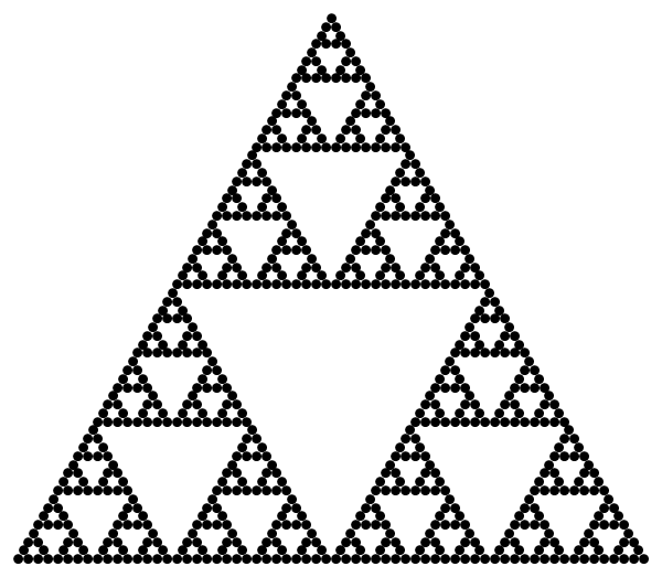
These images look basically the same. Not surprising since they're both point-based. But I gander the distinction between these two algorithms may have been more than just an issue of curiousity 20 years ago. I still remember my first computer, the alien-processored TI-85, chugging away furiously for a good half a minute before the triangle became clear.

Notice that this specific algorithm is actually just a minor modification of the triangle-in-triangle algorithm. The difference is that polygon vertices are here rendered as points. This modification is possible because of Mathematica's symbolic semantics. The symbol Polygon is meaningless until it's processed by the Graphics function. Until then, we can perform structural operations such as replacing it by the Point symbol. In fact the following is completely valid:

axiom = triangle[{{0, 0}, {1, Sqrt[3]}/2, {1, 0}}];

next[prev_] := prev /. triangle[{p1_, p2_, p3_}] :> {
     triangle[{p1, (p1 + p2)/2, (p1 + p3)/2}],
     triangle[{p2, (p2 + p3)/2, (p1 + p2)/2}],
     triangle[{p3, (p1 + p3)/2, (p2 + p3)/2}]};

draw[n_] := Graphics[Nest[next, N@axiom, n] /.  triangle :> Polygon ];

triangle here doesn't have any meaning, ever, until we replace it:

triangle :> Polygon

:

triangle :> Line

:

triangle[pts_] :> Line[RandomChoice[pts, RandomInteger[{2, 3}]]]

:

triangle[pts_] :> Disk[Mean[pts], 1/2^(n + 1)]

:

triangle[pts_] :> Sphere[Append[Mean[pts], 0], 1/2^(n + 1)]

:

Sidenote. What do you get when you methodically build a Lisp on top of symbolic replacement semantics? You get the Mathematica language, of which Mathematica and Mathics appear to be the only incarnations.

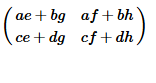
Let's say you forgot how to multiply matrices. Well, just type in some symbols and see the results empirically:

{{a, b}, {c, d}} . {{e, f}, {g, h}} // MatrixForm

If that's still confusing, you can use strings, colored text, graphics, images, etc. instead of symbols. In fact if you have a Tron zapper you can even zap your cat into Mathematica and have him fill up one of those matrix slots, for the advancement of science.

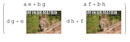
kitty = WolframAlpha["cat picture", "PodImages"][[2]];

(* see http://mathematica.stackexchange.com/a/8291/950 *)
text = First[First[ImportString[ExportString[
      Style["IM IN UR MATRIX...", FontFamily -> "Impact"], "PDF"]]]];

sym = Framed[Overlay[{kitty,
     Graphics[{EdgeForm[Black], White, text}, ImageSize -> 150,
     PlotRangePadding -> 0]}], FrameStyle -> LightGray];

{{a, b}, {Magnify[sym, 1/2], d}} . {{e, f}, {g, h}} // MatrixForm

There's poor Mr. Scruples. Our neighbor will miss him.

The exponential identity for the Pascal matrix is not difficult to understand based on the series definition of the exponential function:

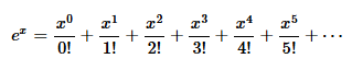
You could work out the matrix arithmetic by hand, or you could do this:

power[n_, p_] := MatrixPower[
    DiagonalMatrix[ToString /@ Range[n], -1], p] // MatrixForm;

Grid[Partition[Table[power[6, p], {p, 1, 6}], 3]] /. 0 -> "\[CenterDot]"

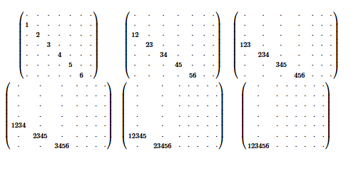
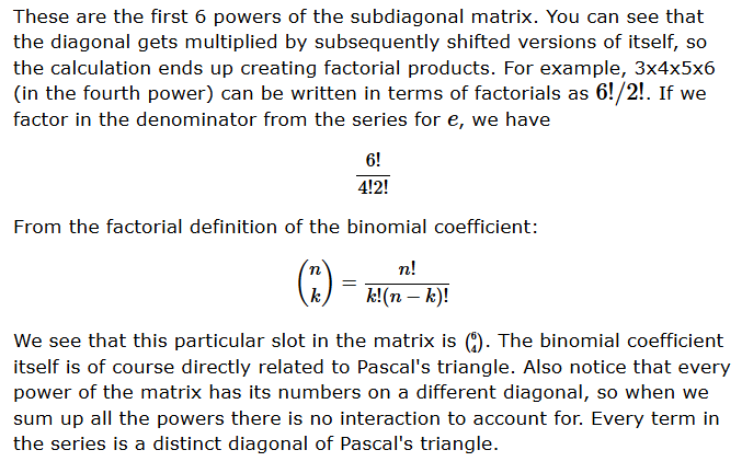
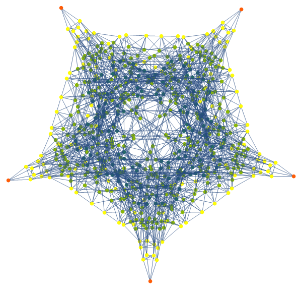
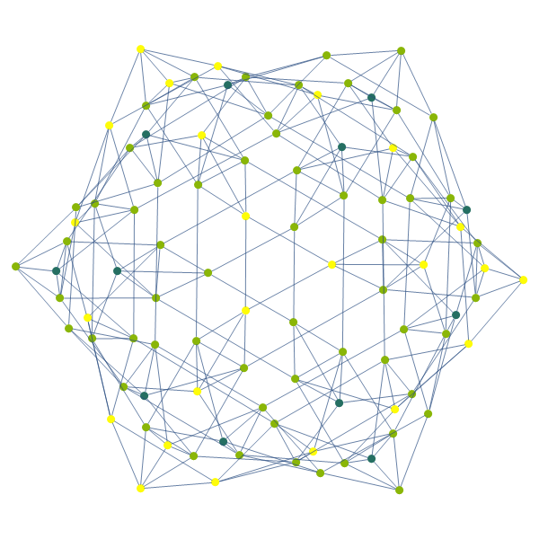
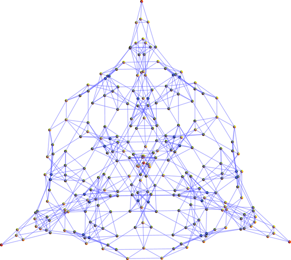
Powers of matrices have a well-known interpretation in terms of graph walks/probabilities. I didn't find anything interesting along this line though. What about graphs represented by the Sierpinski matrix itself?

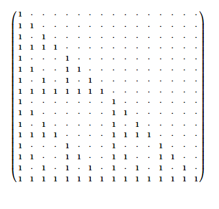
Those were more interesting:

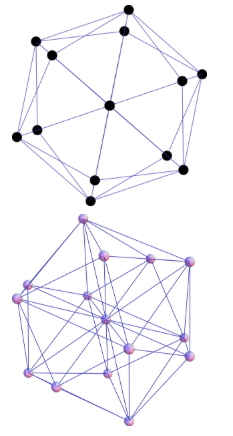
graph[n_] := GraphPlot3D[
   Mod[Array[Binomial, {n, n}, 0], 2],
   Method -> "HighDimensionalEmbedding", Boxed -> False,
   VertexRenderingFunction -> ({White, Sphere[#, .05]} &),
   PlotStyle -> {Thick, Hue[2/3, 2/3, 2/3]}];

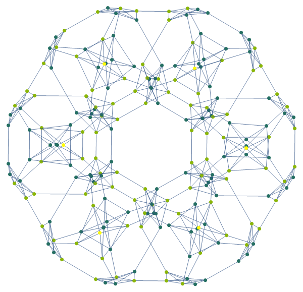
Note this is a 3D graph layout. It has some pretty symmetries. I did some tiresome work trying to figure out what polyhedron it might be.

Tooltip[PolyhedronData[#], #] & /@ Select[
  PolyhedronData[], PolyhedronData[#, "VertexCount"] == 14 &]

After much time, I find. It's the tetrakis hexahedron:

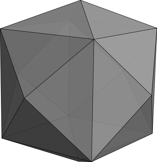
Graphics3D[{Opacity[.94], FaceForm[Gray],
  PolyhedronData["TetrakisHexahedron", "Faces"]},
 Lighting -> "Neutral", Boxed -> False]

I'm certain it's this particular figure because we can just build a graph from its vertex data and then do a graph isomorphism check. And look, we can run this polyhedron grapherizer willy-nilly allabouts, like on the Archimedean solids:

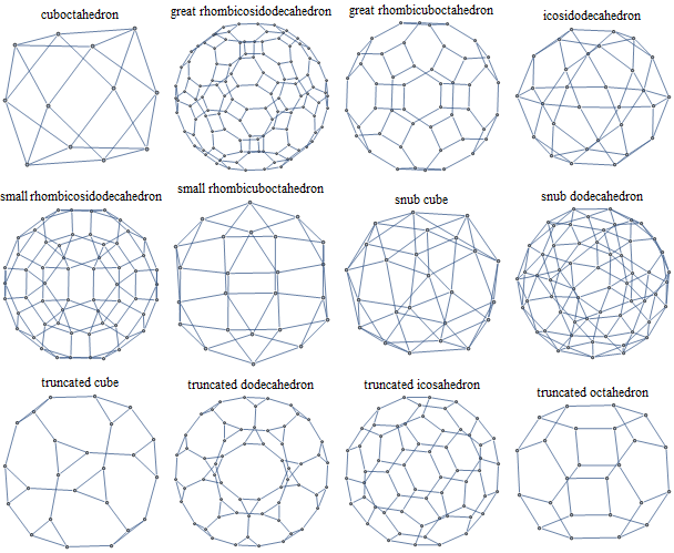
polyGraph[poly_, options___] :=
  Graph[UndirectedEdge @@@ PolyhedronData[poly, "EdgeIndices"], options];

sierpinskiMatrixGraph[n_, options___] := Module[{a},
   (*symmetrize and remove self-loops to allow general isomorphism
   comparison. note that we remove the "inner" vertex since
   we're comparing the "external" geometry as rendered*)
   a = Mod[Array[Binomial, {n, n}, 1], 2];
   AdjacencyGraph[a + Transpose[a] /. 2 -> 0, options]];

IsomorphicGraphQ[polyGraph["TetrakisHexahedron"], sierpinskiMatrixGraph[14]]
IsomorphicGraphQ[polyGraph["CumulatedCube"], sierpinskiMatrixGraph[14]]

Grid[Partition[#, 4]] &[
  polyGraph[#, PlotLabel -> PolyhedronData[#, "Name"]] & /@
   PolyhedronData["Archimedean"]]

Here are the first few powers of the Sierpinski matrix:

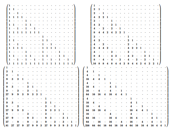
power[n_, p_] := MatrixPower[
   Mod[Array[Binomial, {n, n}, 0], 2], p];

Grid[Partition[#, 2]] &@
 Table[
  MatrixForm[power[16, p] /. 0 -> "\[CenterDot]"],
  {p, 1, 4}]

There's a lot of patterns here. For one, the powers of the Sierpinski matrix are Sierpinski matrices! This isn't necessarily interesting though. The powers of a triangular matrix are going to be triangular. But the numbers follow a curious sequence of powers. For example, in the third power we have the sequence {1, 3, 3, 9, 3, 9, 9, 27, 3, ... }. And this sequence occurs in every column and every row of the matrix, if you hop over the zeros. We can normalize the powers to find:

power[n_, p_] := MatrixPower[
   Mod[Array[Binomial, {n, n}, 0], 2], p];

MatrixForm /@ Table[
  IntegerExponent[power[16, p], p] /. Infinity -> "\[CenterDot]",
  {p, 2, 4}]

This is the sequence in terms of the exponent, and it applies to each power of the Sierpinski matrix, including the first power. For example, 3 to the power of each of {0, 1, 1, 2, 1, 2, 2, 3, 1, ...} is {1, 3, 3, 9, 3, 9, 9, 27, 3, ...}. This power sequence appears in OEIS as the number of ones in the binary representation of n, among other descriptions.

Here is a totally practical application of all of this. A pretty array of buttons:

power[n_, p_] := MatrixPower[Transpose@Reverse@
     Mod[Array[Binomial, {n, n}, 0], 2], p];

Grid[Partition[#, 4]] &@
 With[{m = "you, are now infused, with, the power of, dot, dot, dot... "},
  Array[Function[p,
    Button[Rotate[#, -Pi/4], Speak[m <> ToString[p]]] &@
     Rasterize@MatrixPlot[IntegerExponent[power[2^p, 4], 10],
       ImageSize -> 94, Frame -> None, PlotRangePadding -> 0]],
   8]] 

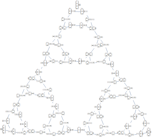
The Towers of Hanoi is a variation on the sticks-in-holes game where instead of putting sticks in holes, you put holes around sticks. Thus the game is ultimately a quaint philosophical remark on the roles of the sexes. But for our purposes there is a claim on the internets that the states of the game form Sierpinski triangle-like graphs:

validQ[s_state] := And @@ Less @@@ s;

(*do all physically possible moves. remove invalid moves afterward.*)
neighbors[states : {__state}] := Select[#, validQ] &@
   DeleteDuplicates@Flatten@
     Table[Module[{st2 = st},

       If[Length[st2[[from]]] > 0,
        PrependTo[st2[[to]], st2[[from, 1]]];
        st2[[from]] = Rest[st2[[from]]]];

       If[st2 =!= st && validQ[st2],
        Sow@UndirectedEdge[st, st2]];

       st2], {st, states}, {to, Length[st]}, {from, Length[st]}];

toStyle[expr_] := expr /. s_state :> (
     Property[Tooltip[s, MatrixForm /@ List @@ s],
      VertexStyle -> {EdgeForm[None],
        ColorData[3][1 + Length[s] - Count[s, {}]]}]);

hanoiGraph[s_, options___] := Module[{vertices, edges, n},
   n = Count[s, _Integer, Infinity];
   {vertices, {edges}} = Reap[Nest[neighbors, {s}, 2^n]];

   SetAttributes[UndirectedEdge, Orderless];
   Graph[toStyle[vertices], DeleteDuplicates[edges],
    options(*,GraphLayout->"SpringEmbedding"*)(*,
    VertexShapeFunction->(Style[#,7,Black]&@
    Text[Row[MatrixForm/@List@@#2],#1]&)*)]];

hanoiGraph[state[{}, {}, Range[4]],
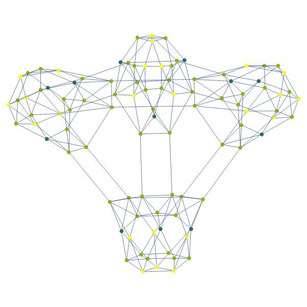
 Epilog -> Inset[Rotate[Style["F-", 300, Bold, Red, Opacity[.65]], Pi/7]]]

Which, as you can see, is a lie if I've ever seen one (internets, you are now on notice). Then again, if you fiddle with the layout and you squint a bit, you can kinda see it, but it's the sort of Sierpinski triangle that Maddox would stamp a huge red F over. To be clear, each vertex represents a single state of the game, and vertices are connected if there is a legal move between those states.

The nice thing about this algorithm is that at each step it just blindly constructs all possibilities, which is easy, and then afterwards removes the ones that aren't valid, which is also easy. Point being it works in broad strokes. And at the end of it we have a map to follow if we ever get stuck. You can do this sort of thing for all sorts of things, like say Rubik's cube. Though I don't know if the combinatorics are favorable in its case. The Towers of Hanoi can be played with more than three sticks:

hanoiGraph[state[{}, {}, {}, Range[4]]]

:

hanoiGraph[state[{}, {}, {}, {}, Range[4]]]

:

hanoiGraph[state[{}, {}, Range[3], Range[3]]]

:

hanoiGraph[state[{}, {}, {1}, Range[3]]]

:

hanoiGraph[state[{}, {}, {2}, Range[3]]]

hanoiGraph[state[{}, {}, {3}, Range[3]]]

:

validQ[s_state] := And @@ Equal @@@ s;
hanoiGraph[state[{}, {}, ConstantArray[1, 5]]]

:

validQ[s_state] := And @@ LessEqual @@@ s;
hanoiGraph[state[{}, ConstantArray[2, 3], ConstantArray[1, 3]]]

:

validQ[s_state] := And @@ Equal @@@ s;
hanoiGraph[state[{}, ConstantArray[2, 3], ConstantArray[1, 3]]]

:

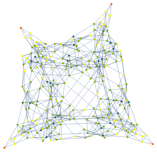
"WHAT THE HELL IS THAT", you say. Indeed, it's messy because it's a low-D rendering. We can also play variations of the game that allow multiple holes of the same diameter, or variations where we adjust the rules a bit. In higher dimensions you can see the structure better:

validQ[s_state] := And @@ Less @@@ s;

(*do all physically possible moves. remove invalid moves afterward.*)
neighbors[states : {__state}] := Select[#, validQ] &@
   DeleteDuplicates@Flatten@
     Table[Module[{st2 = st},

       If[Length[st2[[from]]] > 0,
        PrependTo[st2[[to]], st2[[from, 1]]];
        st2[[from]] = Rest[st2[[from]]]];

       If[st2 =!= st && validQ[st2],
        Sow@UndirectedEdge[st, st2]];

       st2], {st, states}, {to, Length[st]}, {from, Length[st]}];

hanoiGraph[s_, options___] := Module[{vertices, edges, n},
    n = Count[s, _Integer, Infinity];
    {vertices, {edges}} = Reap[Nest[neighbors, {s}, 2^n]];

    SetAttributes[UndirectedEdge, Orderless];
    Graph[DeleteDuplicates[edges]]];

toStyle3D[g_] := Module[{st = VertexList[g][[#2]]},
    Tooltip[{ColorData[3][1 + Length[st] - Count[st, {}]],
      Opacity[1], Sphere[#1, .045]}, MatrixForm /@ List @@ st]] &;

hanoiGraph3D[s_, options___] := Module[{g = hanoiGraph[s]},
   GraphPlot3D[g,
    Method -> "SpringElectricalEmbedding",
    VertexRenderingFunction -> toStyle3D[g], options, Boxed -> False,
    PlotStyle -> {Lighter[Blue](*,Opacity[.5]*)}]];

{vv, vp} = {{0, 0, 1}, {2, 0, 0}};
Animate[
 hanoiGraph3D[state[{}, {}, {}, Range[4]],
  Lighting -> "Neutral", SphericalRegion -> True,
  ViewVertical -> Dynamic[vv], Boxed -> False,
  ViewPoint -> Dynamic[RotationTransform[\[Theta], vv][vp], (vp = #1) &]],
 {\[Theta], 2 Pi, 0}, SynchronousUpdating -> False]

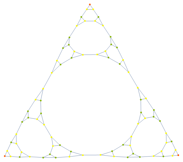
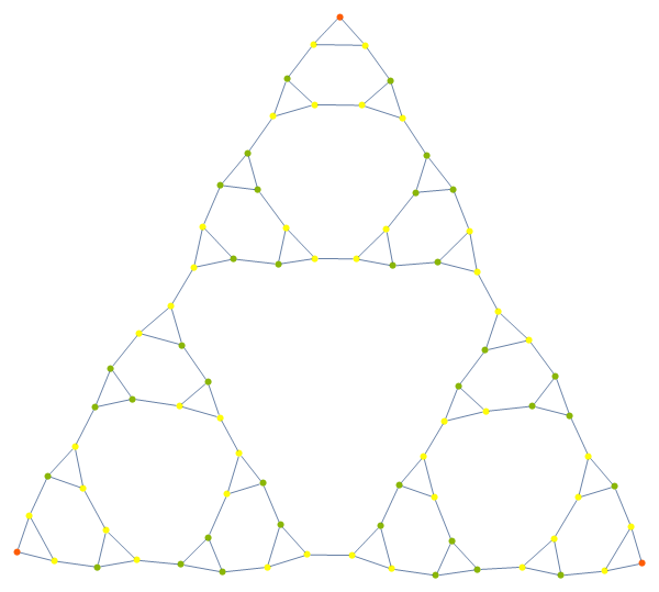
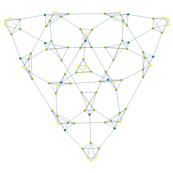
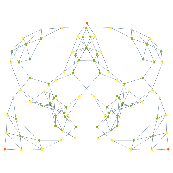
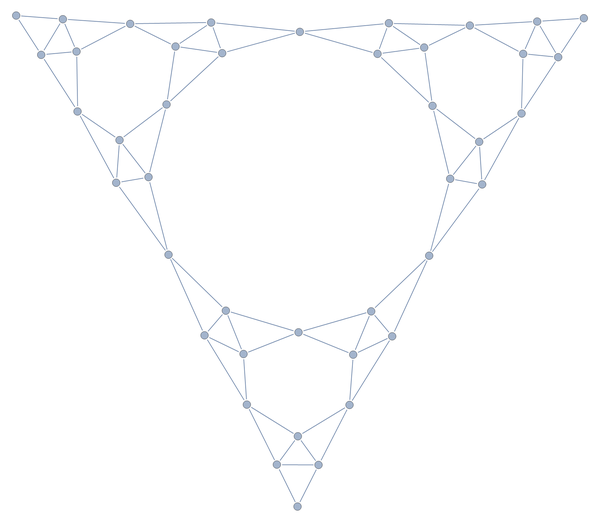
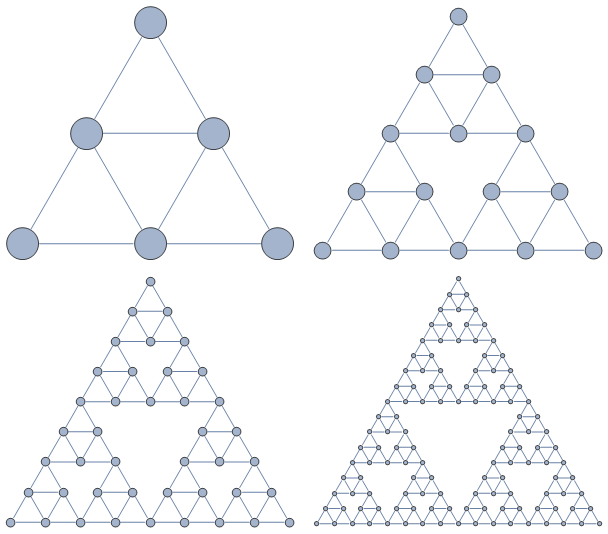
Although the 3-stick Hanoi graphs merely resemble Sierpinski graphs, it would be folly to ignore that resemblance given the thread of recursion that runs through both. We can create Sierpinski graphs easily, by once again reusing our polygon-in-polygon approach and this time replacing the Polygon[{p1, p2, p3}] expression with {p1 <-> p2, p2 <-> p3, p3 <-> p1}:

axiom = Polygon[{{0, 0}, {1, Sqrt[3]}/2, {1, 0}}];

next[prev_] := prev /. Polygon[{p1_, p2_, p3_}] :> {
     Polygon[{p1, (p1 + p2)/2, (p1 + p3)/2}],
     Polygon[{p2, (p2 + p3)/2, (p1 + p2)/2}],
     Polygon[{p3, (p1 + p3)/2, (p2 + p3)/2}]};

draw[n_] := Graph@Flatten@
    Nest[next, N@axiom, n] /. Polygon[pts_] :>
     Sequence @@ UndirectedEdge @@@ Partition[pts, 2, 1, 1];

axiom = Polygon[{{0, 0}, {1, Sqrt[3]}/2, {1, 0}}];

next[prev_] := prev /. Polygon[{p1_, p2_, p3_}] :> {
     Polygon[{p1, (p1 + p2)/2, (p1 + p3)/2}],
     Polygon[{p2, (p2 + p3)/2, (p1 + p2)/2}],
     Polygon[{p3, (p1 + p3)/2, (p2 + p3)/2}]};

(*Orderless attribute not necessary here. but it causes the particular permutation
 of the edge list that results in the particular layout*)

(*triple-click on "DynamicSetting" below, Right-click -> Evaluate in Place*)
DynamicSetting[SetterBar[1, {SetAttributes, ClearAttributes}]][UndirectedEdge, Orderless];
draw[n_] := Graph[#, VertexSize -> .05, GraphLayout -> "SpringEmbedding"] &@
    Flatten@Nest[next, N@axiom, n] /. Polygon[pts_] :>
     Sequence @@ UndirectedEdge @@@ Partition[pts, 2, 1, 1];

g = draw[5]
GraphPlot3D[g, VertexRenderingFunction -> None,
   PlotStyle -> Hue[2/3, 2/3, 2/3(*,1/2*)],
   Method -> "SpringEmbedding", Boxed -> False]

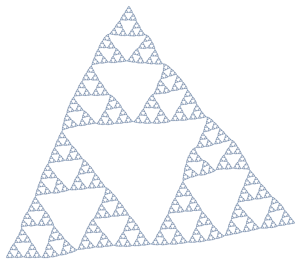
There's the Sierpinski triangle I know and love; the graph of. You might think it doesn't look good. But you don't realize it's a Sierpinski triangle wearing a cape made of Sierpinski triangles. Not only does it not not look good, it looks completely badass. Because we're using the coordinates of the points as vertices, we can straightforwardly recover the regular Sierpinski layout:

axiom = Polygon[{{0, 0}, {1, Sqrt[3]}/2, {1, 0}}];

next[prev_] := prev /. Polygon[{p1_, p2_, p3_}] :> {
     Polygon[{p1, (p1 + p2)/2, (p1 + p3)/2}],
     Polygon[{p2, (p2 + p3)/2, (p1 + p2)/2}],
     Polygon[{p3, (p1 + p3)/2, (p2 + p3)/2}]};

draw[n_] := Module[{edges},
   edges = Flatten@Nest[next, N@axiom, n] /. Polygon[pts_] :>
      Sequence @@ UndirectedEdge @@@ Partition[pts, 2, 1, 1];

   Graph[edges, VertexCoordinates -> VertexList[Graph[edges]],
    VertexSize -> .25]];

The point of spending 1 or 2 LOC's worth of developer time to convert our geometric Sierpinski triangle into a graph is so that we can ask questions about the graph. Like for example, what are its Hamiltonicness and Eulerity quotients? What is the average degree of the graph, in Celsius? In Kelvin? Frankly most of these questions are boring, and I don't really know anything about graphs. But here is a picture of the line graphs of the first few Sierpinski iterations:

axiom = Polygon[{{0, 0}, {1, Sqrt[3]}/2, {1, 0}}];

next[prev_] := prev /. Polygon[{p1_, p2_, p3_}] :> {
     Polygon[{p1, (p1 + p2)/2, (p1 + p3)/2}],
     Polygon[{p2, (p2 + p3)/2, (p1 + p2)/2}],
     Polygon[{p3, (p1 + p3)/2, (p2 + p3)/2}]};

draw[n_] := Module[{edges},
   edges = Flatten@Nest[next, N@axiom, n] /. Polygon[pts_] :>
      Sequence @@ UndirectedEdge @@@ Partition[pts, 2, 1, 1];

   Graph[edges, VertexCoordinates -> VertexList[Graph[edges]],
    VertexSize -> .25]];

g = draw[2];
LineGraph[g]

cycle = RandomChoice[{FindHamiltonianCycle, FindEulerianCycle}][g][[1]];

Animate[
 HighlightGraph[g, Graph[cycle[[1 ;; n]]],
  EdgeShapeFunction -> (Line[#1] &),
  VertexShapeFunction -> None,
  GraphHighlightStyle -> "DehighlightHide"],
 {n, 1, Length[cycle], 1}, AnimationRate -> 1]

axiom = Polygon[{{0, 0}, {1, Sqrt[3]}/2, {1, 0}}];

next[prev_] := prev /. Polygon[{p1_, p2_, p3_}] :> {
     Polygon[{p1, (p1 + p2)/2, (p1 + p3)/2}],
     Polygon[{p2, (p2 + p3)/2, (p1 + p2)/2}],
     Polygon[{p3, (p1 + p3)/2, (p2 + p3)/2}]};

sierpinskiGraph[n_] := Graph@Flatten@
     Nest[next, N@axiom, n] /. Polygon[pts_] :>
    Sequence @@ UndirectedEdge @@@ Partition[pts, 2, 1, 1];

dg = Mean[VertexDegree[sierpinskiGraph[8]]];

(*if live in us, above comes out in farenheit, so have to convert*)
us = Graphics[CountryData["UnitedStates", "Polygon"], ImageSize -> 8000];
If[Rasterize[us] === Rasterize[Show[us, Graphics[{PointSize[0], Point[Reverse@FindGeoLocation[]]}]]],
 WolframAlpha[ToString[dg, InputForm] <> " degrees f in celcius", {{"Result", 1}, "NumberData"}],
 dg]

Also the minimal zig zag of the triangle, notable because it looks like a bunch of resistors (no doubt the inspiration for certain papers). And its minimal criss cross. I don't really see anything though. Do you see anything? I don't see anything. These graphs just vertices and edges to me.

They do raise a question though. What game (or what anything) does the Sierpinski graph represent? I wasn't able to produce the Sierpinski triangle from any variation of the Hanoi game beyond the first couple of trivial iterations. In any case, through the extensive research I've done here I've found that layered graph layouts are pretty:

validQ[s_state] := And @@ Less @@@ s;
neighbors[states : {__state}] := Select[#, validQ] &@
   DeleteDuplicates@Flatten@
     Table[Module[{st2 = st},
       If[Length[st2[[from]]] > 0,
        PrependTo[st2[[to]], st2[[from, 1]]];
        st2[[from]] = Rest[st2[[from]]]];
       If[st2 =!= st && validQ[st2],
        Sow@UndirectedEdge[st, st2]];
       st2], {st, states}, {to, Length[st]}, {from, Length[st]}];

hanoiGraph[s_] := Module[{vertices, edges, n},
   n = Count[s, _Integer, Infinity];
   {vertices, {edges}} = Reap[Nest[neighbors, {s}, 2^n]];
   SetAttributes[UndirectedEdge, Orderless];
   Graph[DeleteDuplicates[edges]]];

axiom = Polygon[{{0, 0}, {1, Sqrt[3]}/2, {1, 0}}];
next[prev_] := prev /. Polygon[{p1_, p2_, p3_}] :> {
     Polygon[{p1, (p1 + p2)/2, (p1 + p3)/2}],
     Polygon[{p2, (p2 + p3)/2, (p1 + p2)/2}],
     Polygon[{p3, (p1 + p3)/2, (p2 + p3)/2}]};

(*certain layout depends on this ordering*)
(*next[prev_]:=prev/.Polygon[pts_]:>(
Polygon[ScalingTransform[1/2{1,1},#][pts]]&/@pts);*)

sierpinskiGraph[n_] := Graph@Flatten@
    Nest[next, N@axiom, n] /. Polygon[pts_] :>
     Sequence @@ UndirectedEdge @@@ Partition[pts, 2, 1, 1];

draw[g_] := LayeredGraphPlot[g,
   EdgeRenderingFunction -> ({CapForm["Round"], Line[#]} &),
   VertexRenderingFunction -> None,
   PlotStyle -> {Thickness[.01], Black}];

draw /@ {hanoiGraph[state[{}, {}, Range[3]]], sierpinskiGraph[3]}

Chaos

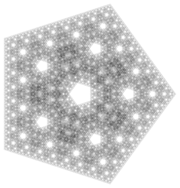
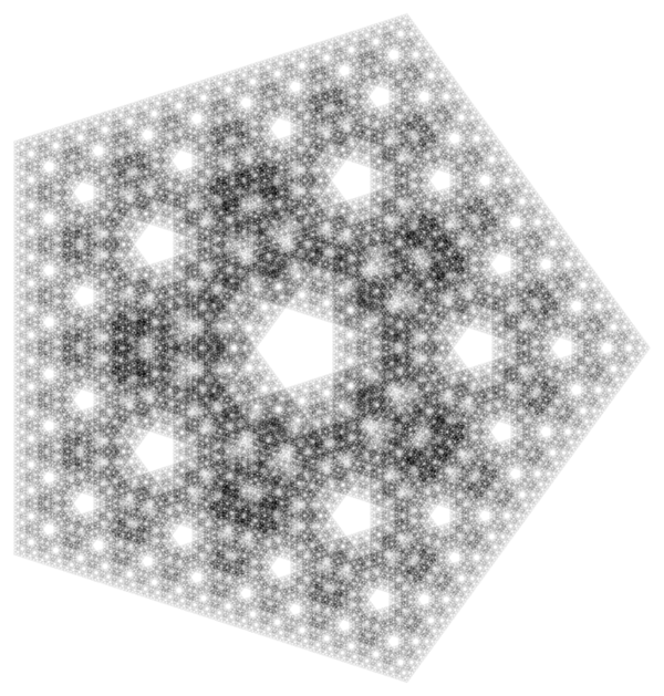
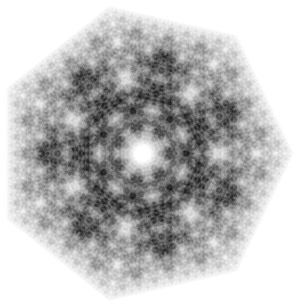
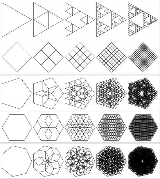
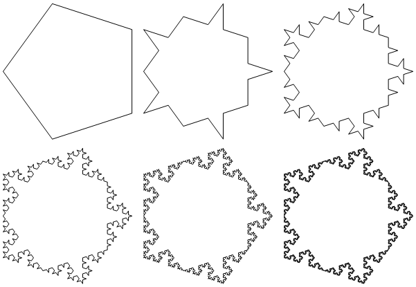
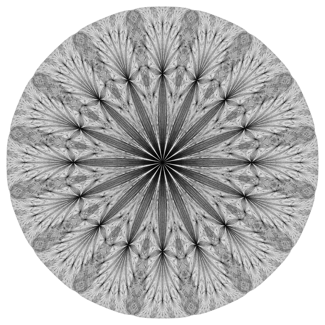
One of the nice things about the chaos game algorithm is that we can easily generalize it to more than three points. To begin with, we can place equiangular points on a circle using cos and sin (see also my screwing around with polygons).

draw[v_, numPoints_] := Module[{vertices},
  vertices = {Cos[#], Sin[#]} & /@ (2 Pi Range[v]/v);

  Graphics[{PointSize[0], Opacity[.1],
    Point[FoldList[(#1 + #2)/2 &, N@{0, 0},
      RandomChoice[N@vertices, numPoints]]]}]];

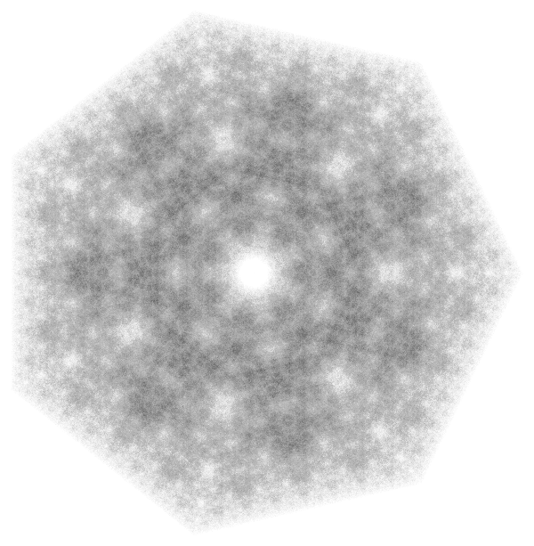
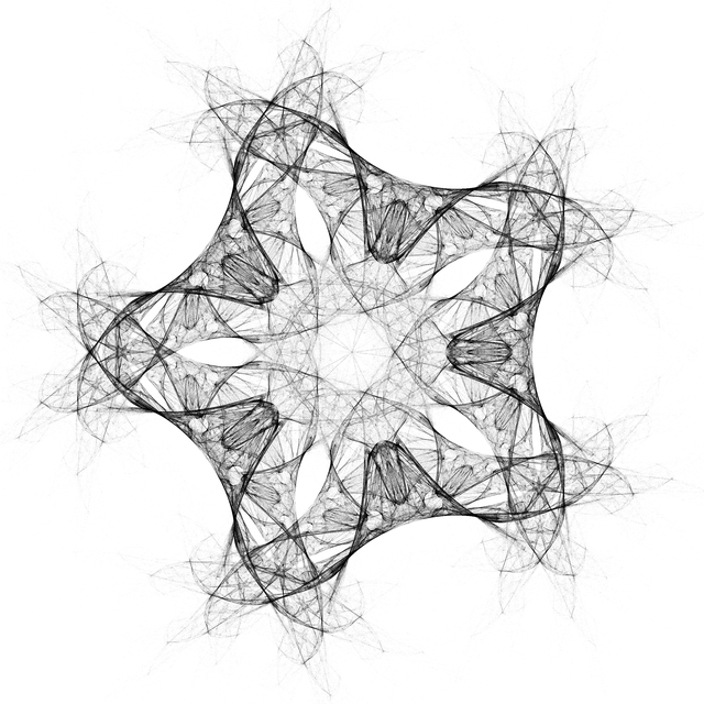
These are drawn with 10 million points. The last two are drawn with 50 million points. The key to the quality here is giving the points transparency so that varying degrees of overlap/nearness form different shades. Higher vertex counts clearly have some structure, but it becomes blurry for one reason or another. You might be able to pull out the structure better with a more methodical approach and some image trickery.

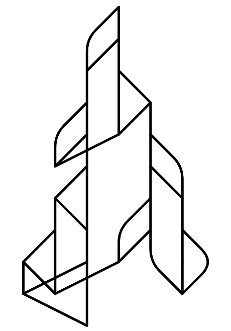
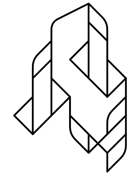
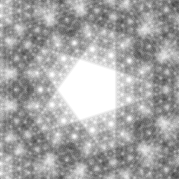
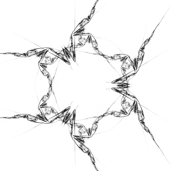
If you play around with pentagons in a vector editor (Mathematica itself has basic vector editing capabilities), you will find this figure:

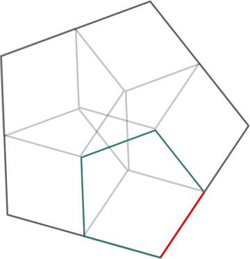
I've highlighted one of the inner pentagons. You can see that this figure reproduces the faded stellation pattern in the center of the chaos game rendition. So the chaos game algorithm remains consistent in this geometric fashion: At each vertex of the figure, attach a copy of the larger figure, but with sidelength one-half of the original (note the red edge in the above image).

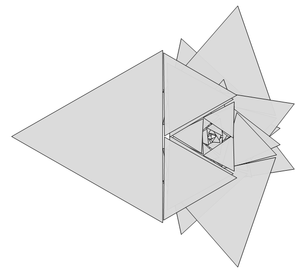
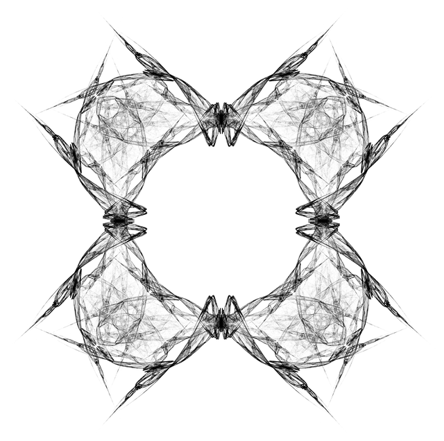
This also explains why the 4-vertex rendering is a block. And since we now have the geometric rule, we can turn to an explicit geometric construction to see if we can make the structure of these chaos games clearer. After some hiccups, I was able to get something working:

SetAttributes[toXY, Listable];
toXY[z_] := {Re[z], Im[z]};

ring[c_, r_, 0] := c;
ring[c_, r_, depth_] := Module[{zs},
   zs = c + r E^(I 2 Pi Range[3]/3);
   ring[c + # Normalize[# - c], r/2., depth - 1] & /@ zs];

Graphics[Rotate[{Opacity[.95], LightGray, EdgeForm[Black],
   Polygon /@ toXY /@ Level[ring[0, 1, 5], {-2}]}, Pi]]

draw[v_, n_] := Module[{ring},
   ring[c_, r_, depth_] := Module[{ps},
     ps = c + r {Cos[#], Sin[#]} & /@ (2. Pi Range[v]/v);

     If[depth == 0, Polygon[ps],
      ring[(c + #)/2, r/2, depth - 1] & /@ ps]];

   Graphics[{Transparent,
     EdgeForm[{Opacity[.28], Black}],
     ring[0., 1., n]}]];

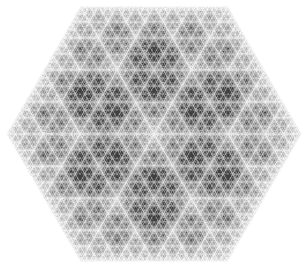
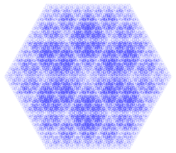
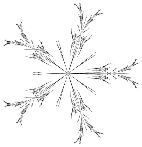
The snowflake has all sorts of symmetries, probably because 6 = 2 × 3. It even has 3D grids and cubes. It's an infinite cubic matryoshka snowflake. And there is a lot of amazing detail in these drawings.

At this point I should mention that all of the code snippets on this page are self-contained. If you have Mathematica you can copy-paste this and start producing these figures.

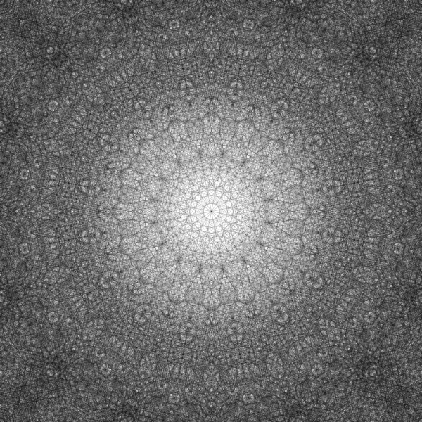
The chaos game has another generalization. Instead of moving halfway between the active point and the randomly-chosen vertex, we can move 1/3rd of the way, or 3/2 of the way, etc:

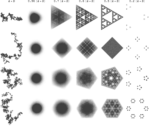
draw[v_, df_, numPoints_: 10000] := Module[{vertices},
   vertices = {Cos[#], Sin[#]} & /@ (2 Pi Range[v]/v);

   Graphics[{PointSize[0], Opacity[.5],
     Point[FoldList[df, N@{0, 0},
       RandomChoice[N@vertices, numPoints]]]}]];

functions = Function[r, (#1 + #2) r &] /@ {1, .96, .7, .6, .5, .2};

Grid[Join[
  {TraditionalForm[#[a, b]] & /@ functions},
  Table[draw[v, df], {v, 3, 6}, {df, functions}]]]

In the case where we're just adding the numbers, we get a normal n-directional random walk. Of course, the geometric approach has its own similar generalization:

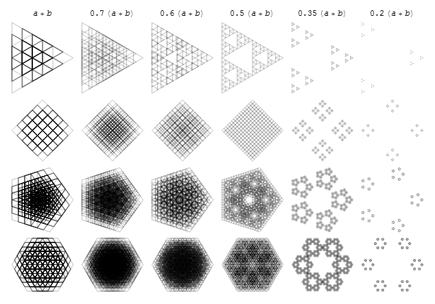
draw[v_, df_, n_] := Module[{ring},
   ring[c_, r_, depth_] := Module[{ps},
     ps = c + r {Cos[#], Sin[#]} & /@ (2. Pi Range[v]/v);

     If[depth == 0, Polygon[ps],
      ring[(c + #)/2, df[0, r], depth - 1] & /@ ps]];

   Graphics[{Transparent,
     EdgeForm[{Opacity[.26], Black}],
     ring[0., 1., n]}]];

functions = Function[r, (#1 + #2) r &] /@ {1, .7, .6, .5, .35, .2};

Grid[Join[
  {TraditionalForm[#[a, b]] & /@ functions},
  Table[draw[v, df, 4], {v, 3, 6}, {df, functions}]]]

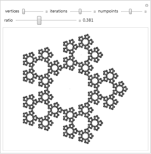
One of the things you might try to do, if you're me, is adjust the ratio until the corners match up:

drawGeom[v_, ratio_, n_] := Module[{ring},
   ring[c_, r_, depth_] := Module[{ps},
     ps = c + r {Cos[#], Sin[#]} & /@ (2. Pi Range[v]/v);

     If[depth == 0, Polygon[ps],
      ring[(c + #)/2, r ratio, depth - 1] & /@ ps]];

   Graphics[{Transparent,
     EdgeForm[{Opacity[.28], Black}],
     ring[0., 1., n]}]];

drawChaos[v_, ratio_, numPoints_] := Module[{vertices},
   vertices = {Cos[#], Sin[#]} & /@ (2 Pi Range[v]/v);

   Graphics[{PointSize[0], Opacity[.5],
     Point[FoldList[(#1 + #2) ratio &, N@{0, 0},
       RandomChoice[N@vertices, numPoints]]]}]];

With[{
  verticesC = Control[{vertices, 3, 8, 1, ImageSize -> Tiny}],
  iterationsC = Control[{iterations, 0, 8, 1, ImageSize -> Tiny}],
  numPointsC = Control[{numpoints, 0, 100000, 1, ImageSize -> Tiny}]},

 Manipulate[Overlay[{
    drawGeom[vertices, ratio, iterations],
    drawChaos[vertices, ratio, numpoints]}],
  Row[{verticesC, iterationsC, numPointsC}, " "],
  {{ratio, .5}, 0, 1, Appearance -> "Labeled"},
  Alignment -> Center]]

Look! There are Koch snowflake figures that form in the negative space. The boundary becomes snowflaked. A Koch snowflake can easily be made with an L-system construction:

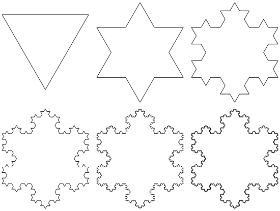
axiom = {F, right[2], F, right[2], F};
rules = F -> {F, left[1], F, right[2], F, left[1], F};
conversions = {F -> forward, dir_[n_] :> ConstantArray[dir, n]};

(*state transformations*)
forward[{z_, theta_}] := {z + E^(I theta), theta};
left[{z_, theta_}] := {z, theta + 2 Pi/6};
right[{z_, theta_}] := {z, theta - 2 Pi/6};

draw[n_] :=
  Module[{program, zs},
   program = Flatten[Nest[# /. rules &, axiom, n] /. conversions];
   zs = First /@ ComposeList[program, {0., 0.}];
   Graphics[{Thin, Line[{Re[#], Im[#]} & /@ zs]}]];

Grid[Partition[#, 3]] &[draw /@ Range[0, 5]]

axiom = {F, right[1], F, right[1], F, right[1], F, right[1], F};
rules = F -> {F, left[1], F, right[2], F, left[1], F};
conversions = {F -> forward, dir_[n_] :> ConstantArray[dir, n]};

(*state transformations*)
forward[{z_, theta_}] := {z + E^(I theta), theta};
left[{z_, theta_}] := {z, theta + 2 Pi/5};
right[{z_, theta_}] := {z, theta - 2 Pi/5};

draw[n_] :=
  Module[{program, zs},
   program = Flatten[Nest[# /. rules &, axiom, n] /. conversions];
   zs = First /@ ComposeList[program, {0., -Pi/10.}];
   Graphics[{Thin, Line[{Re[#], Im[#]} & /@ zs]}]];

Grid[Partition[#, 3]] &[draw /@ Range[0, 5]]

With some minoradjustments we get our pentagonal snowflake. If we do the same procedure for the hexagonal chaos game we get the familiar triangular snowflake. All of the geometries seem to create Koch snowflakes, which makes sense given that indentations are triangles.

Of course, there are much more interesting generalizations we can come up with than simple ratios:

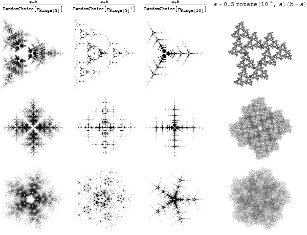
draw[v_, df_, numPoints_: 1000] := Module[{vertices},
   vertices = {Cos[#], Sin[#]} & /@ (2 Pi Range[v]/v);

   Graphics[{PointSize[0], Opacity[.15],
     Point[FoldList[df, N@{0, 0},
       RandomChoice[N@vertices, numPoints]]]}]];

rotate = RotationTransform;
functions = {
   (#1 + #2)/RandomChoice[Prime[Range[3]]] &,
   (#1 + #2)/RandomChoice[Prime[Range[3]]!] &,
   (#1 + #2)/RandomChoice[Prime[Range[10]]] &,
   #1 + .5 rotate[10. Degree, #1][#2 - #1] &};

Grid[Join[
  {TraditionalForm[Trace[#[a, b]][[2]]] & /@ functions},
  ParallelTable[draw[v, df], {v, 3, 5}, {df, functions}]]]

Some of these drawings remind me of the kind of fractal scattering found in the more deterministic algorithms. I wonder what kind of relation there is. The best distance function I found was logarithm-based:

game = Compile[{{v, _Integer}, {wowzerz, _Real}, {numPoints, _Integer}},
   Module[{diff, vertices},
    vertices = {Cos[#], Sin[#]} & /@ (2 Pi Range[v]/v);

    (*distance function is Clip[(a+b)Log[EuclideanDistance[a,b]+wowzerz]*)
    FoldList[(
       diff = #2 - #1;(*note each of these is an x-y pair*)
       Clip[(#1 + #2) Log[Sqrt[diff.diff] + wowzerz], 1.1 {-2, 2}]) &,
     {0, 0}, RandomChoice[vertices, numPoints]]]];

Graphics[{PointSize[0], Opacity[.08],
  Point[game[5, .8, 300000]]}(*,PlotRange->1.15*)]

All of these images are from the same distance function. The 'holes' on the inward-folded leaves of this one are interesting. It's like a fractal Klein bottle thing goin on there. If my computer was worth more than my car, as it some day will be, I would burn a lot of lightning-sequestered power in my mad scientist laboratory in the process of rendering different distance functions. There's a lot of pretty pictures in these simple chaos games. As it stands all this lightning is going to waste.

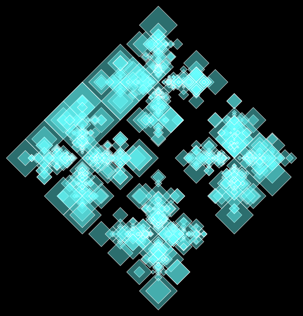
The geometric approach, not one to have been served, decides to go Tron:

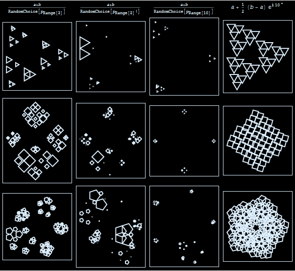
draw[v_, df_, n_] := Module[{ring},
   ring[c_, r_, depth_] := Module[{zs},
     zs = c + r E^(I 2. Pi Range[v]/v);

     If[depth == 0, Polygon[{Re[#], Im[#]} & /@ zs],
      ring[(c + #)/2, df[0, r], depth - 1] & /@ zs]];

   Framed[Graphics[{Transparent,
      EdgeForm[{Thick, LightBlue}],
      ring[0., 1., n]}], FrameStyle -> LightBlue]];

functions = {
   (#1 + #2)/RandomChoice[Prime[Range[3]]] &,
   (#1 + #2)/RandomChoice[Prime[Range[3]]!] &,
   (#1 + #2)/RandomChoice[Prime[Range[10]]] &,
   #1 + (1/2) (#2 - #1) E^(I 10. Degree) &};

Framed[Grid[Join[
   {TraditionalForm[Trace[#[a, b]][[2]]] & /@ functions},
   Table[draw[v, df, 3], {v, 3, 5}, {df, functions}]]],
 Background -> Black, BaseStyle -> LightBlue]

draw[v_, df_, n_] := Module[{ring},
   ring[c_, r_, depth_] := Module[{ps},
     ps = c + r {Cos[#], Sin[#]} & /@ (2. Pi Range[v]/v);

     If[depth == 0, Polygon[ps],
      ring[(c + #)/2, df[0, r], depth - 1] & /@ ps]];

   Graphics[{EdgeForm[White], Opacity[.4],
     RGBColor[.4, 1, 1], ring[0., 1., n]}]];

Show[(*repeatedly draw to cover more possibilities*)
 draw[4, (#1 + #2)/RandomChoice[Prime[Range[4]]] &,
    RandomChoice[{.1, 1.5} -> {2, 3}]] & /@ Range[20],
 Background -> Black, ImageSize -> 600]

Or Asteroids. Same thing.

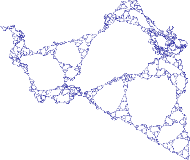
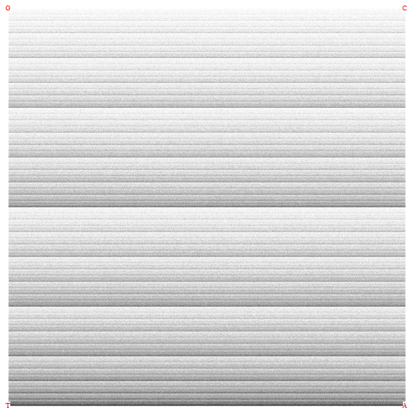
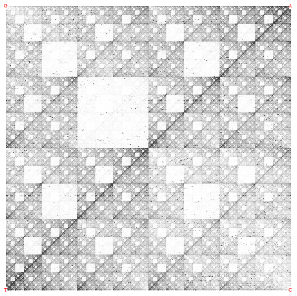
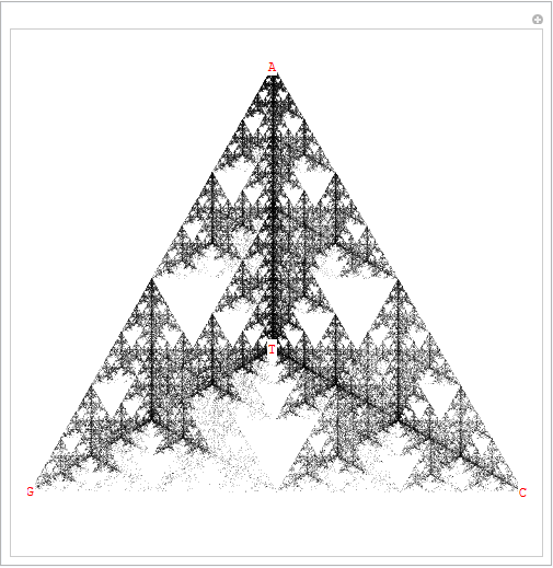
The most interesting place I've seen the chaos game is in genetics. The idea is that instead of randomly picking the vertex at each step, you let the letters of the genetic code pick for you. There are 4 letters in DNA: A, T, G, C. So you run a chaos game with 4 vertices. If some sequence of DNA is AAAATC, your active point will approach the point labeled A 4 times, then it will approach the T point, then the C point.

If the DNA sequence is completely random, you will just recreate our beautiful block, which I have named the Charcoal Diamond:

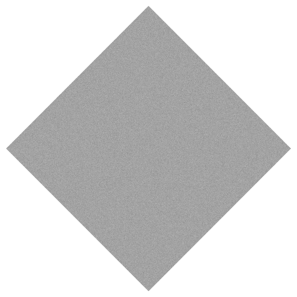
But what you get is not random, as this chaos plot shows:

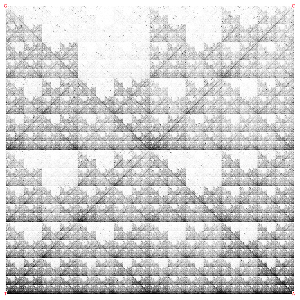
coords = N@{"A" -> {1, -1}, "T" -> {-1, -1}, "G" -> {-1, 1}, "C" -> {1, 1}};
dat = Characters[GenomeData[{"ChromosomeX", {28000000, 36000000}}]] /. coords;

draw[data_] := Graphics[{PointSize[0], Opacity[.01],
    Point[FoldList[(#1 + #2)/2 &, N@{0, 0}, data]]},
   Epilog -> Style[Text @@@ coords, Red, Background -> White]];

draw[dat]

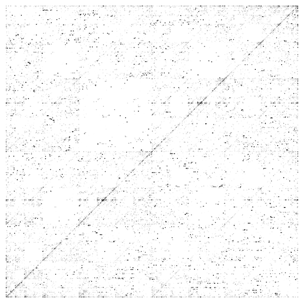
This is a chaos game plot of an arbitrarily-chosen 8 million basepair sequence from our chromosome X (for scale, a typical protein is encoded in only a few hundred basepairs). You might insensibly think this happens because the letters occur with different frequencies, but that's not the case. The following is a chaos game plot of a sequence that was randomly generated over the same statistical frequencies as the above sequence:

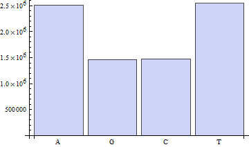
chars = Characters[GenomeData[{"ChromosomeX", {28000000, 36000000}}]];
tallies = Tally[chars];
BarChart[Last /@ tallies, ChartLabels -> First /@ tallies]

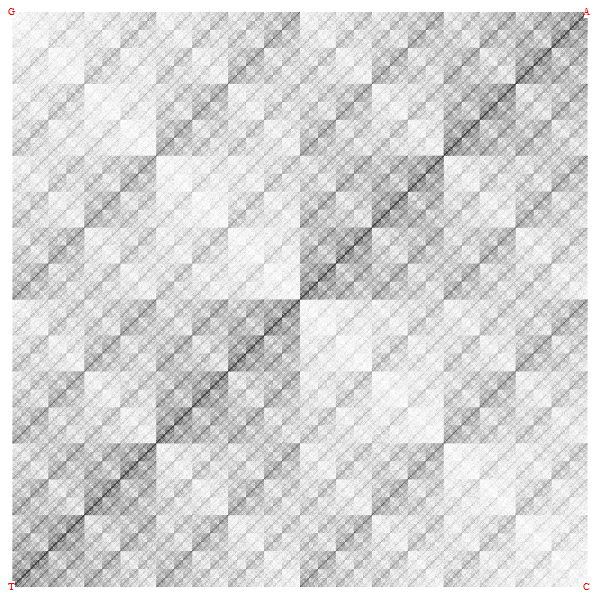
coords = N@{"A" -> {1, 1}, "T" -> {-1, -1}, "G" -> {-1, 1}, "C" -> {1, -1}};
dat = Characters[GenomeData[{"ChromosomeX", {28000000, 36000000}}]] /. coords;

scale = 2;
grid = Tuples[Range[{-1, -1}, {1, 1} - 2^-scale, 2^-scale]];
color = If[Mod[Plus @@ #*2^scale, 2] == 1,
    Blend[{Lighter@Purple, Yellow}],
    Blend[{Lighter@Blue, Red}]] &;

overunder = Graphics[{Opacity[.25],
    {color[#], Rectangle[#, # + 2^-scale]} & /@ grid}];

draw[data_] := Show[overunder,
   Graphics[{PointSize[0], Opacity[.06],
     Point[FoldList[(#1 + #2)/2 &, N@{0, 0},
       RandomChoice[data, Length[data]]]]}],
   overunder, PlotRange -> 1, ImageSize -> {600, 600}];

draw[dat] // Rasterize

coords = N@{"A" -> {1, -1}, "T" -> {-1, -1}, "G" -> {-1, 1}, "C" -> {1, 1}};
dat = Characters[GenomeData[{"ChromosomeX", {28000000, 36000000}}]] /. coords;

draw[data_] := Graphics[{PointSize[0], Opacity[.01],
    Point[FoldList[(#1 + #2)/2 &, N@{0, 0}, RandomChoice[data, Length[data]]]]},
   Epilog -> Style[Text @@@ coords, Red, Background -> White]];

draw[dat]

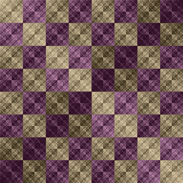
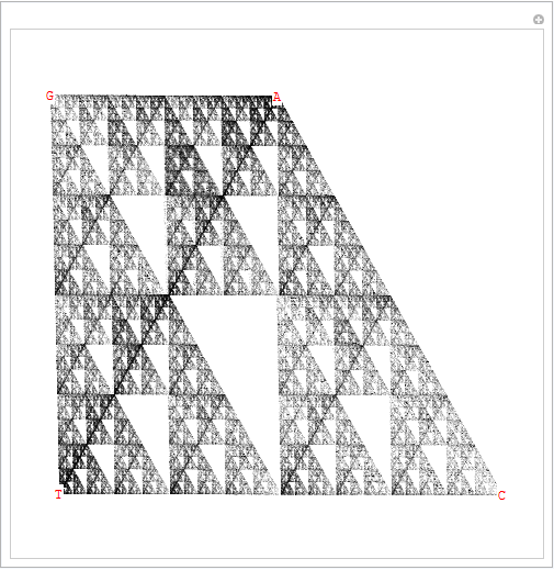
The letters do occur in different frequencies, but that doesn't make any interesting patterns. If you move the letters around you get a pattern related in this case to the fact that the frequencies are bilateral, but otherwise it's just a glorified chessboard. And look what happens when we do the same vertex movearounding for our genetic code:

coords = N@{"A" -> {1, 1}, "T" -> {-1, -1}, "G" -> {-1, 1}, "C" -> {1, -1}};
dat = Characters[GenomeData[{"ChromosomeX", {28000000, 36000000}}]] /. coords;

draw[data_] := Graphics[{PointSize[0], Opacity[.01],
    Point[FoldList[(#1 + #2)/2 &, N@{0, 0}, data]]},
   Epilog -> Style[Text @@@ coords, Red, Background -> White]];

draw[dat]

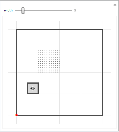
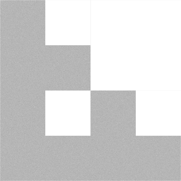
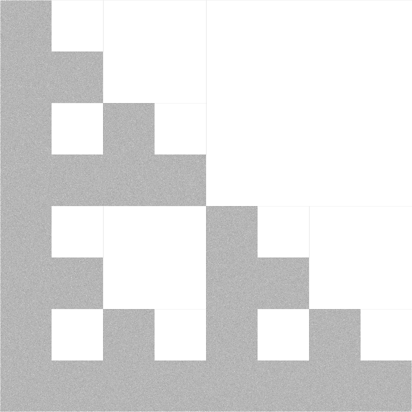
The original paper does a good job explaining how the chaos plot is something of a "fractal subsequence histogram." Assume your active point is anywhere in the entire square, and the next move is toward the bottom-left corner. Because you move halfway toward that corner (instead of, say, only one third or one fifth of the way), you will land inside that corner's quadrant regardless of where your point was to begin with.

Furthermore, you can apply this argument to subquadrants. It's easy to see this if you "work backwards." The formula for going from the current active point toward the next vertex is

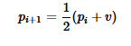
By the DeLorean transform, we can go backwards like this:

So, reversing all the points in a particular subquadrant:

Manipulate[Module[{delorean, preimage, pt1, pt2},
  pt1 = ptc - width;
  pt2 = ptc + width;

  delorean[x_] := 2 x - coord;
  preimage = delorean /@ Tuples[Range[pt1, pt2, .025]];

  Graphics[{
    EdgeForm[{Thickness[.01], Darker[Gray, .4]}],
    {Transparent, Rectangle[{-1, -1}, {1, 1}]},
    {LightGray, Rectangle[pt1, pt2]},
    {Gray, Point[preimage]}},
   PlotRange -> 1.2, GridLines -> Automatic,
   GridLinesStyle -> Lighter[Gray, .8]]],

 {{width, .25}, 0, .5, 2.^-3},
 {{ptc, {-.75, -.25}}, Locator},
 {{coord, {-1, -1}}, Locator,
  Appearance -> Style["\[FilledSquare]", Red]}]

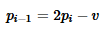
You can see here that for all the points which were just ordered to move toward the little red dot in the bottom-left corner, those that landed in the gray square had to have come from the top-left quadrant of the main square (the region with gray dots). So for the points in that gray region, we not only know that they were ordered to move toward the bottom-left vertex in the last step, but also that they were ordered to move toward the top-left vertex in the step before that.

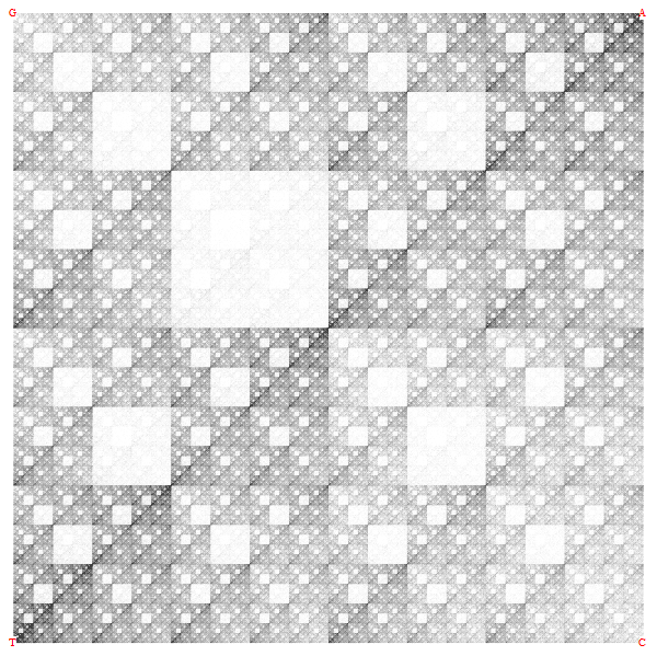
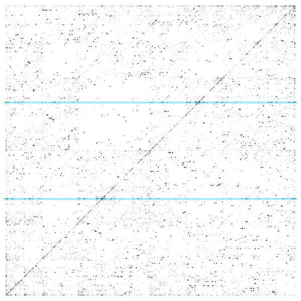
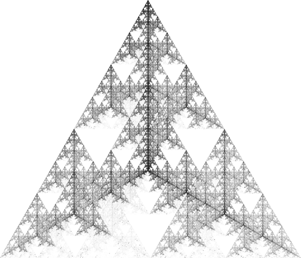
And so on. The points in this little gray region were ordered to move previously toward the bottom-left, and before that the top-left, and before that the bottom-right. All points in that square have that history. So going back to our genetic chaos plot:

What those big holes mean is that CG is a rare sequence. As we just saw, a point can only get to that big empty square by coming from the bottom-right quadrant and going toward the top-left vertex. And since that square is so empty, there are rarely any points that are available to go toward other subsquares, such as this one, and so on.

This accounts for the texture of the first chaos plot as well. It just looks more wacked out because the CG vertices are adjacent, so the empty squares touch each other and create those staggered serrations. A simple histogram confirms our suspicions of CG Paucity — a.k.a. biology's Dark Energy:

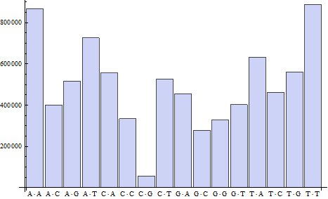
chars = Characters[GenomeData[{"ChromosomeX", {28000000, 36000000}}]];
tallies = Sort[Tally[Partition[chars, 2, 1]]];
BarChart[Last /@ tallies, ChartLabels -> CenterDot @@@ First /@ tallies]

If you sample subsequences instead of individual letters, and use those samples to simulate a genetic sequence, what's the smallest subsequence-sampling size you can get away with while still faithfully reproducing the texture of the chaos plot?

Asked differently, what length of subsequence is it that accounts for the texture of the chaos plot? Here is a graph of our DNA letters with pair-wise sequences labeled by probability:

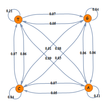
chars = Characters[GenomeData[{"ChromosomeX", {28000000, 36000000}}]];
tallies = Sort[Tally[Partition[chars, 2, 1]]];
sum = Total[Last /@ tallies];
stats = {Rule @@ #1, #2/sum} & @@@ tallies;

With[{r = .05},
 edgeF[pts_List, e_] := Arrow[pts, r];
 edgeF[pts_List, h_[a_, a_]] := Scale[Arrow[pts, r/.3], .3, pts[[1]]];
 vertexF = {EdgeForm[Opacity[.5]], Disk[#1, r], Darker[Gray, .7],
    Style[Text[#2, #1], 13, Bold, FontFamily -> "Comic Sans MS"]} &;
 edgeLabels = #1 -> Style[Round[#2, .01], 12, Bold] & @@@ stats;]

Graph[First /@ stats, EdgeLabels -> edgeLabels,
 EdgeStyle -> Directive[{Thick, Opacity[.56]}],
 VertexShapeFunction -> vertexF, VertexStyle -> Orange,
 EdgeShapeFunction -> edgeF, PlotRangePadding -> .1]

This is a graph of what's called a Markov chain, but don't quote me on the formalities. (Mathematica 9 has built-in Markov whatitswhats, but I'm using version 8). The point is we can generate a sequence whose letter-to-letter statistics are the same as those of our original DNA by following the graph probaballistically:

getStats[data_] := Module[{tallies, sum},
   tallies = Tally[Partition[data, 2, 1]];
   sum = Total[Last /@ tallies];
   {Rule @@ #1, #2/sum} & @@@ tallies];

draw[data_, options___] := Graphics[{PointSize[0], Opacity[.01],
    Point[FoldList[(#1 + #2)/2 &, N@{0, 0}, data]]}, options,
   Epilog -> Style[Text @@@ coords, Red, Background -> White]];

chars = Characters[GenomeData[{"ChromosomeX", {28000000, 36000000}}]];
stats = getStats[chars];

Do[With[{weights =
    Rule @@ Transpose@Cases[stats, {letter -> to_, p_} :> {N[p], to}]},
  next[letter] := RandomChoice[weights]],
 {letter, DeleteDuplicates[stats[[All, 1, 1]]]}]

coords = N@{"A" -> {1, 1}, "T" -> {-1, -1}, "G" -> {-1, 1}, "C" -> {1, -1}};
pseudoDat = NestList[next, "A", Length[chars]] /. coords;

draw[pseudoDat]

You can see that, while similar, the fake plot immediately stands out as too Hollywood compared to the verisimilous beauty of the real data. The most notable distinction between them, besides the grain, is the dark diagonal that crosses A and T in the real plot, presumably because those two letters have a lot of interplay. That it's not replicated by our pseudosequence may mean there are a relatively large amount of ATA, TAT subsequences.

So it looks like subsequences of length 2 aren't sufficient. We could generalize our Markovizer, but what I think is actually interesting here is the grain. We can do some image processing to see if we can bring it out:

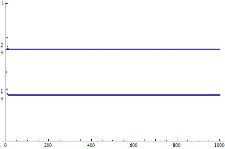
ListPlot[FoldList[(#1 + #2)/2 &, 1,
  Mod[Range[1000], 2]], PlotRange -> 1,
 Ticks -> {Automatic, Range[0, 1, 1/3]}]

getStats[data_] := Module[{tallies, sum},
   tallies = Tally[Partition[data, 2, 1]];
   sum = Total[Last /@ tallies];
   {Rule @@ #1, #2/sum} & @@@ tallies];

draw[data_, options___] := Graphics[{PointSize[0], Opacity[.01],
    Point[FoldList[(#1 + #2)/2 &, N@{0, 0}, data]]}, options];

chars = Characters[GenomeData[{"ChromosomeX", {28000000, 36000000}}]];
stats = getStats[chars];

Do[With[{weights =
    Rule @@ Transpose@Cases[stats, {letter -> to_, p_} :> {N[p], to}]},
  next[letter] := RandomChoice[weights]],
 {letter, DeleteDuplicates[stats[[All, 1, 1]]]}]

coords = N@{"A" -> {1, 1}, "T" -> {-1, -1}, "G" -> {-1, 1}, "C" -> {1, -1}};
pseudoDat = NestList[next, "A", Length[chars] - 1] /. coords;
realDat = chars /. coords;

With[{upsc = 2},
 pseudo = draw[pseudoDat, ImageSize -> upsc 600] // Rasterize;
 real = draw[realDat, ImageSize -> upsc 600] // Rasterize;

 With[{\[Theta] = ColorNegate},
   (ImageSubtract[\[Theta][real], \[Theta][pseudo]] // \[Theta])
     ~MinFilter~1
     ~ImageMultiply~1.1
    (*~ImageAdjust~(9!)*)
    // ImageAdjust]
  ~ImageResize~Scaled[1/upsc]]

chars = Characters[GenomeData[{"ChromosomeX", {28000000, 36000000}}]]; 
tallies = Sort[Tally[Partition[chars, 3, 1]]];
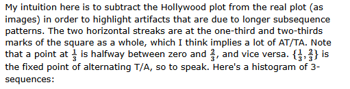
BarChart[Last /@ tallies, ChartLabels -> Column /@ First /@ tallies]

chars = Characters[GenomeData[{"ChromosomeX", {28000000, 36000000}}]];
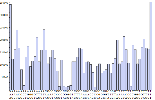
tallies = Sort[Tally[Partition[chars, 5, 1]]];
ListPlot[Cases[tallies, {seq_, count_} :> Tooltip[count, Column[seq]]],
 Axes -> None, Filling -> Axis, PlotRange -> Full]

Which actually just shows a lot of TTT and AAA. Longer subsequence statistics show a similar picture. And of course we can always just do this:

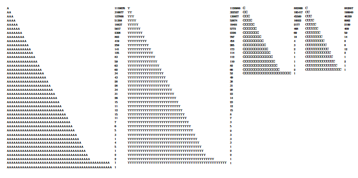
string = GenomeData[{"ChromosomeX", {28000000, 36000000}}];
tallies = Sort[Tally[StringCases[string, ("A" .. | "T" .. | "C" .. | "G" ..)]]];

Grid[Join[
   Sequence @@ Reverse@Sort@
      SplitBy[tallies, StringTake[First[#], 1] &], 2],
  Alignment -> Left] // Magnify[#, 1/2] &

string = GenomeData[{"ChromosomeX", {28000000, 36000000}}];
strings = ParallelTable[Module[{cases =
      StringCases[string, Alternatives @@ cs .., Overlaps -> True]},
    Last@SortBy[cases, StringLength]],
   {cs, Subsets[{"A", "C", "T", "G"}, {2}]}];

Grid[{Tooltip[Short[#], #], StringLength[#]} & /@
  Reverse@SortBy[strings, StringLength], Alignment -> Left]

The longest single-letter run length in this section of DNA is 48 As. The longest string of A-or-T is 222 basepairs long. Quite long, but the longest pairing is actually T/C which has a sequence of length 231. C/G's longest sequence is 34 basepairs long. I wonder what it is about CG. Maybe an unusually (un)useful amino acid or some hydrophobilia issue. I wonder too if these are blanket statistical patterns or if certain quirks are only present, say, in non-coding regions.

You might be wondering why we don't just ask a biologist about these mysteries. The reason is because you're inside a car right now, I'm driving, we're lost, both of us are tourists, and I'm one of those people that would sooner burn hours of gasoline/diesel than ask for directions. You also suspect I might be some kind of criminal, so you're afraid of bringing up the issue. All around it's pretty awkward in here.

We can do a lot better than these static diagrams by giving ourselves the ability to manually movearound the vertices to see if we can find interesting patterns:

coords = N@{"A" -> {1, 1}, "T" -> {-1, -1}, "G" -> {-1, 1}, "C" -> {1, -1}};
chars = Characters[GenomeData[{"ChromosomeX", {28000000, 36000000}}]];

draw[data_, options___] := Graphics[{PointSize[0], Opacity[.1],
    Point[FoldList[(#1 + #2)/2 &, N@{0, 0}, data]]}, options];

Manipulate[
 draw[
  chars[[1 ;; 100000]] /. Thread[First /@ coords -> pts],
  PlotRange -> 1.1],
 {{pts, Last /@ coords}, Locator,
  Appearance -> (Framed[#, BaseStyle -> Red,
       FrameStyle -> None, FrameMargins -> 0,
       Background -> White] & /@ First /@ coords)}]

And a tool that repeatedly applies the DeLorean transform to rebuild the sequence leading up to a region:

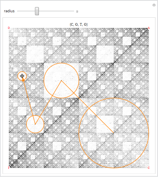
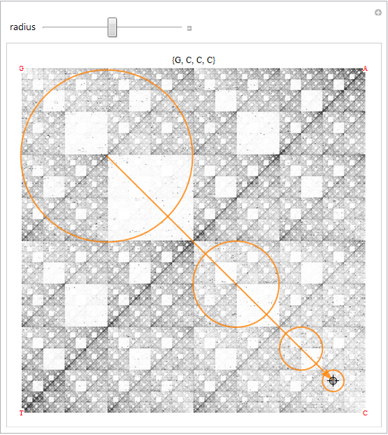
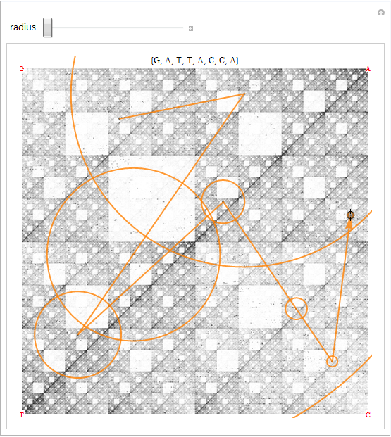
coords = N@{"A" -> {1, 1}, "T" -> {-1, -1}, "G" -> {-1, 1}, "C" -> {1, -1}};
dat = Characters[GenomeData[{"ChromosomeX", {28000000, 36000000}}]] /. coords;
nfLetter = Module[{nf = Nearest[Reverse /@ coords]}, nf[#, 1][[1]] &];

draw[data_, options___] := Graphics[{PointSize[0], Opacity[.01],
    Point[FoldList[(#1 + #2)/2 &, N@{0, 0}, data]]}, options];

background = Raster[Reverse@ImageData@Rasterize@
      draw[dat, PlotRange -> 1, ImageSize -> 600 {1, 1}],
   {{-1, -1}, {1, 1}}];

delorean[p_] := 2 p - (nfLetter[p] /. coords);
Manipulate[Module[{seq, r = 2^radius},
  seq = Most[NestList[delorean, pt, Floor[1/(2 r)]]];

  Graphics[{background, {Darker@Gray, Point[seq]},
    {Orange, Thick, Opacity[.8], Arrow[Reverse[seq]],
     MapThread[Circle, {seq, 2^(radius + 1) r 2^Range[Length[seq]]}]}},
   PlotRange -> 1.015, PlotLabel -> (nfLetter /@ Reverse[seq]),
   Epilog -> Style[Text @@@ coords, Red, Background -> White]]],

 {{radius, -2}, -4, -2, 1},
 {{pt, {-.75, -.25}}, Locator}]

I'm not actually sure how legit the maths of the program are, but there it be. Let's return to our charcoal diamond, here rotated:

drawDiamond[numPoints_] := Graphics[{PointSize[0], Opacity[.01],
    Point[FoldList[(#1 + #2)/2 &, N@{0, 0}, RandomInteger[{0, 1}, {numPoints, 2}]]]},
   ImageSize -> 600, PlotRangePadding -> 0];

diamond = drawDiamond[15000000] // Rasterize;

axiom = {{Transparent, Rectangle[Scaled[{0, 0}], Scaled[{2, 2}]]}, White,
   If[hl, EdgeForm[{Opacity[.1], Green}]], Rectangle[Scaled[{1, 1}], Scaled[{2, 2}]]};

next[prev_] := Translate[Scale[prev, .5], {{-1, 1}, {-1, -1}, {1, -1}}];

Control[{hl, {True, False}}] Control[{n, 0, 10, 1}]
Dynamic[Overlay[{diamond, Graphics[NestList[next, axiom, n],
    ImageSize -> (ImageSize /. AbsoluteOptions[diamond]), PlotRange -> 1]}]]

Imagine we suddenly removed one vertex. That would mean that points can no longer land in that quadrant. Which would mean that no points could go from that quadrant to these subquadrants. Which would mean no points going to these subquadrants. And soon and soforth, until.

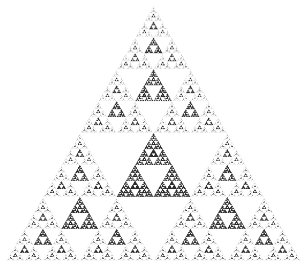
So that explains the holes in the Sierpinski triangle. I call this the "Sierpinski triangle by infinite quadrilateral descent" method of construction. It seems very natural to me, but it raises the question of what these regions in the various deterministic constructions have to do with each other:

draw[n_] := Array[Tooltip[Mod[Binomial[##], 2],
     TraditionalForm[HoldForm[Binomial[##]] == Binomial[##]]] &, {2^n, 2^n}, 0];
proc[a_ /; Length[a] == 2] := a;
proc[arr_] := Module[{l = Length[arr]/2},
   ArrayFlatten@Map[Function[square,
      If[FreeQ[square, Tooltip[1, _]],
       (**)Map[Style[#, Bold, ColorData[3][l]] &, square, {2}],
       (**)proc[square]]], Partition[arr, {l, l}], {2}]];
Style[MatrixForm[proc[draw[5]]], Background -> GrayLevel[.98]]

(To be clear, the chaos game is just an algorithmic tradeoff vs the geometric approach. It is not necessarily doing anything non-deterministic in the larger scheme.) In this case I think the parity/binary explanations are going to be the simplest, though I'm a math noob and I don't see an immediately obvious way of approaching this, if the question even makes sense in the way I seem to be implying. However with some inspiration we can find an iterative angle that seems to me like a kind of multiplication:

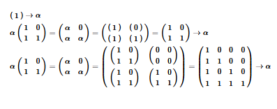
(* minimal *)

iterate[matrix_, power_] := Nest[ArrayFlatten[
     ConstantArray[#, Dimensions[matrix]] matrix] &, 1, power];

draw[matrix_, power_] :=
  ArrayPlot[iterate[matrix, power],
   Frame -> False, PixelConstrained -> 1];

draw[{{1, 0}, {1, 1}}, 10]

matrixInput[Dynamic[m_], Dynamic[rot_]] :=
  Dynamic[Rotate[Deploy[MatrixForm[#, TableSpacing -> {0, 0}]], rot] &@
    Array[(*(*better performance*)Rotate[#,-rot]&@*)
     Checkbox[Dynamic[m[[##]]], {0, 1}] &, Dimensions[m]]];

bg = White;
dims = # -> If[# > 4, Style[#, Red], #] & /@ Range[7];

iterate[matrix_, power_] := Nest[ArrayFlatten[
     ConstantArray[#, Dimensions[matrix]] matrix] &, 1, power];

controls = With[{
    mC = Control[{{m, 2, ""}, dims, ControlType -> PopupMenu}],
    nC = Control[{{n, 2, ""}, dims, ControlType -> PopupMenu}],
    matrixInputC = matrixInput[Dynamic[matrix], Dynamic[rot]],
    colorC = Control[{{color, Black}, ColorSlider}],
    rotC = Control[{{rot, 0, "\[Theta]"}, Pi, -Pi, Pi/16}],
    powerC = Control[{{power, 3}, 1, 4, 1, Appearance -> "Labeled"}],
    opacityC = Control[{{opacity, 1}, 0, 1, ImageSize -> Small}],
    primitiveC = Control[{{primitive, Rectangle[]},
       (# -> Graphics[{color, #}, ImageSize -> 20] &) /@ {
         {PointSize[Tiny], Point[N@{0, 0}]},
         {EdgeForm[None], Disk[N@{0, 0}, .5]},
         Rotate[Scale[Rectangle[], 1./Sqrt[2]], Pi/4],
         Rectangle[]}, SetterBar}],
    backgroundC = Row[{"background   ",
       Framed[ColorSlider[Dynamic[background, (bg = background = #) &],
         AppearanceElements -> "Swatch"], FrameStyle -> Darker[Gray]],
        " ",
       ColorSlider[Dynamic[background, (bg = background = #) &],
        AppearanceElements -> "Spectrum", ImageSize -> Small]}]},

   Row[{
     Column[{
       Row[{mC, "   \[Times]", nC}],
       Row[{"    ", matrixInputC}]}],
     Spacer[40],
     Column[{colorC, rotC, powerC}],
     Column[{backgroundC, opacityC, primitiveC}]}]];

Panel[#, Background -> Dynamic[bg]] &@
 Manipulate[
  If[{m, n} =!= Dimensions[matrix], matrix = PadRight[matrix, {m, n}]];

  With[{primitives = Rotate[#, rot - Pi/2] &@
      Translate[primitive, Position[
        iterate[matrix /. 0 matrix -> {{1}}, power], 1]]},

   Graphics[{Dynamic[EdgeForm[{Opacity[opacity], color}]],
     Dynamic[color], Dynamic[Opacity[opacity]], primitives},
    ImageSize -> {{400, Large}, {400, Large}},
    Background -> Dynamic[background]]],

  Evaluate[controls],

  (*declare variables here for persistence*)
  {{background, bg = White}, ControlType -> None},
  {{matrix, {{1, 0}, {1, 1}}}, ControlType -> None},

  Bookmarks :> {
    "Random" :> (matrix = RandomChoice[{.4, .6} -> {0, 1}, Dimensions[matrix]]),
    "Invert" :> (matrix = BitXor[matrix, 1]),
    "Array Print" :> (With[{p = power, m = matrix, c = color, o = opacity, bg = background},
      CellPrint[ExpressionCell[Defer[
         ArrayPlot[iterate[m, p], Frame -> False, PixelConstrained -> 1,
          ColorRules -> {0 -> bg, 1 -> c /. RGBColor[r_, g_, b_] :> RGBColor[r, g, b, o]}]],
        "Input"]]]),
    "Clear" :> (matrix = 0 matrix)},

  Paneled -> False, SynchronousUpdating -> Automatic,
  SaveDefinitions -> True, LabelStyle -> Darker[Gray], Alignment -> Center]

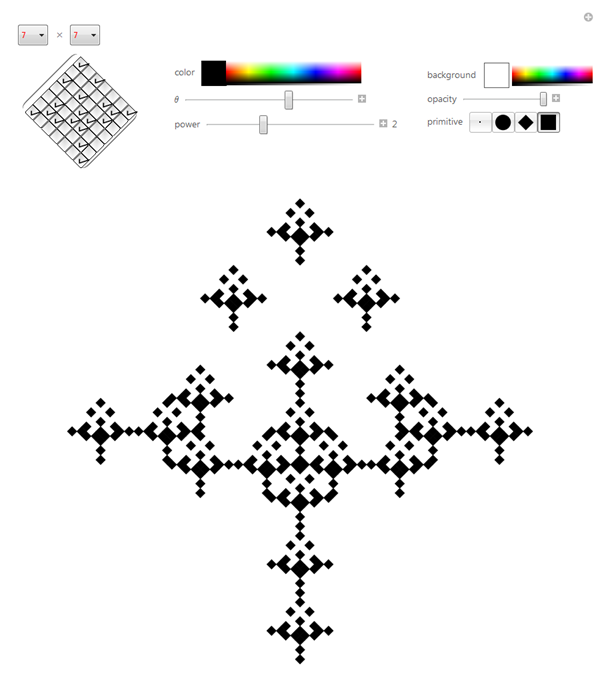
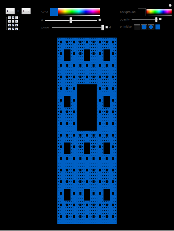
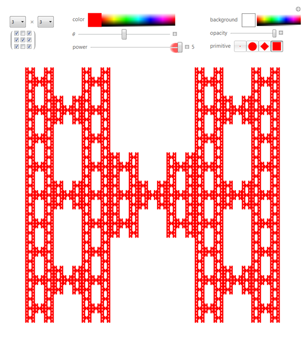
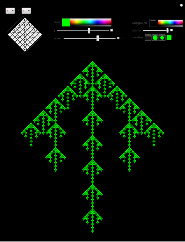
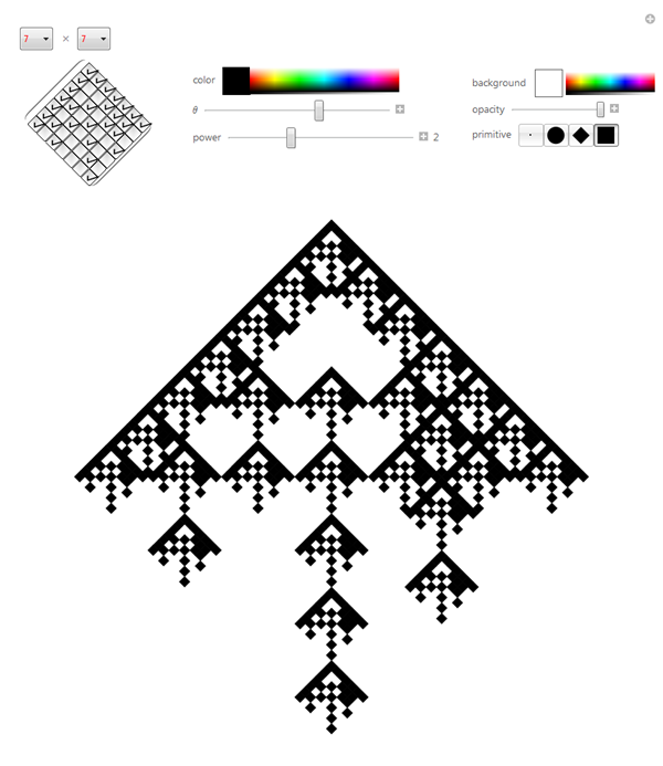
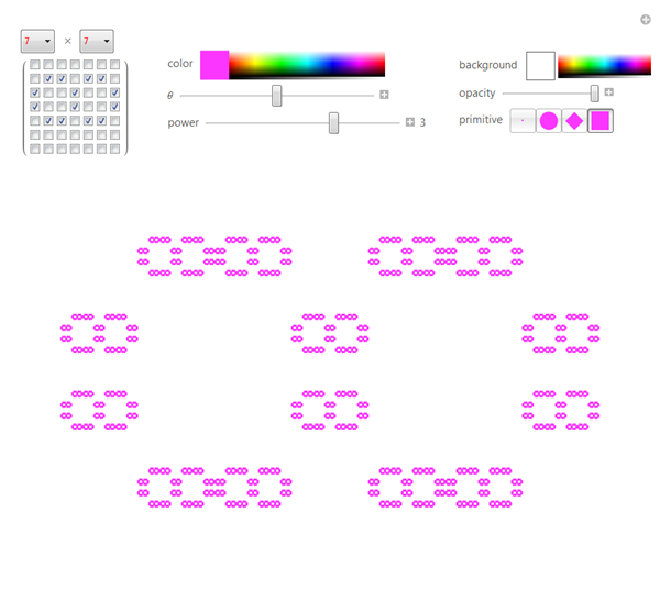
I know what this image reminds you of. Those little candle chandoliers that you hit in Castlevania to make hearts and morning stars come out. I also found The Sierpinski Scream, a letter H that would definitely beat you up if it was human, the up arrow and its Hot Topic-donning offspring, pink infinities made of pink infinities, even the vaunted Sierpinski Chronobracket.

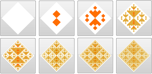
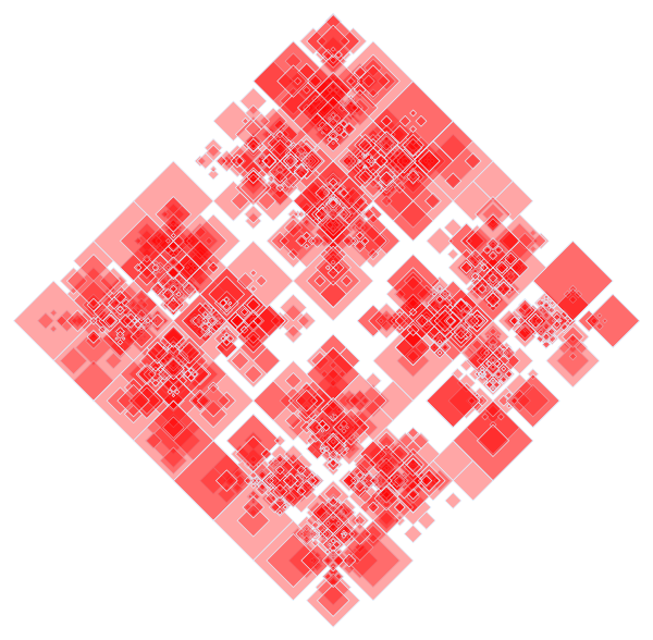
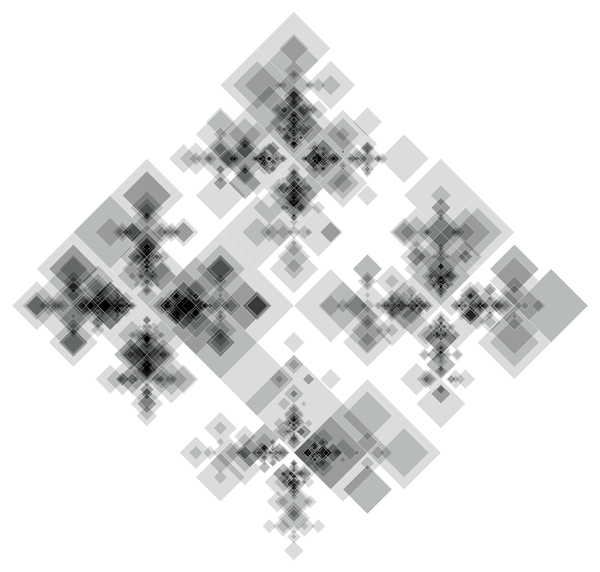
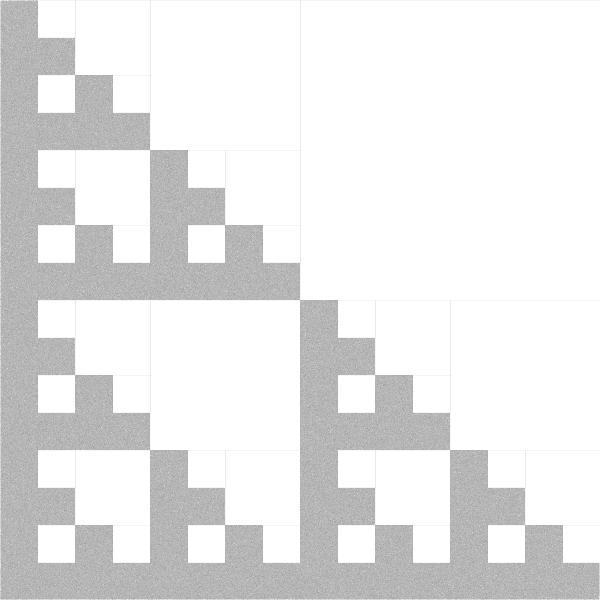
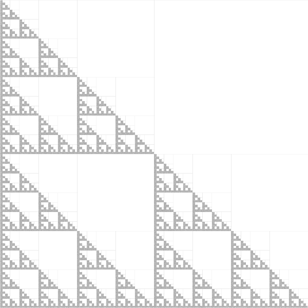
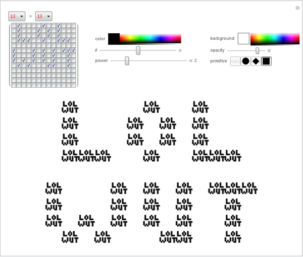
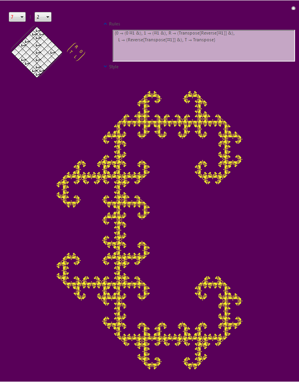
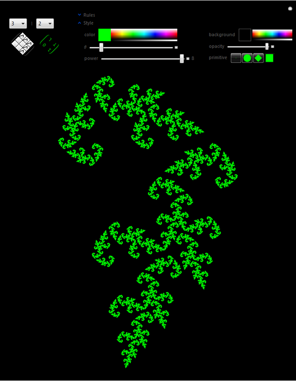
Essentially what we have here in these little matrices is a notation for specifying translations. It's yet another algorithm with different tradeoffs for doing more or less the same thing that our chaos game and geometric algorithms are doing. We can bring this characteristic out by allowing arbitrary rules:

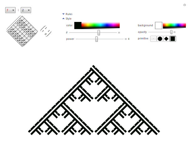
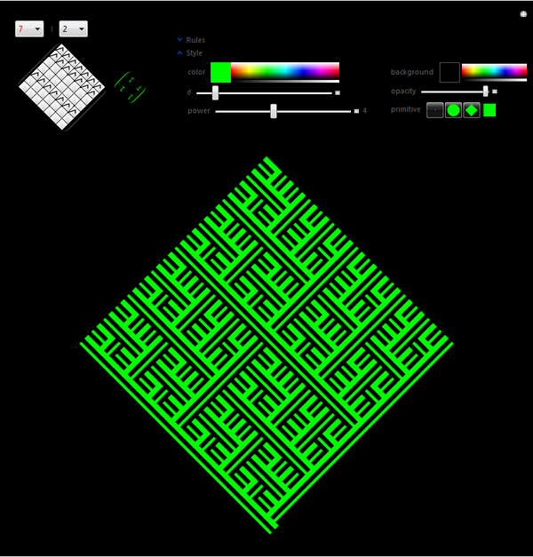
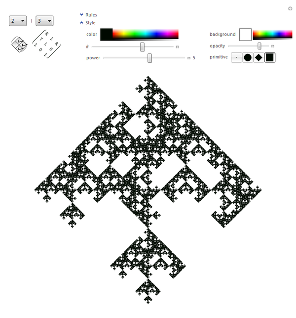
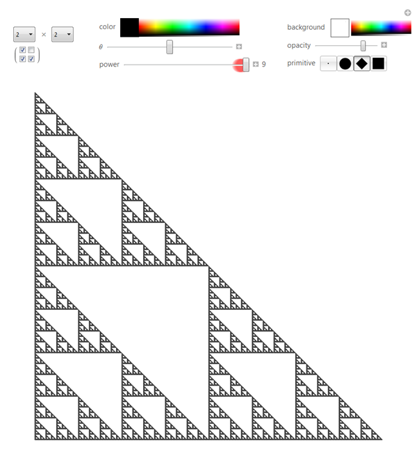
(* minimal *)

iterate[matrix_, power_, matrix1_: {{1}}] := Module[{rules =
     {0 -> (0 # &), 1 -> (# &), T -> Transpose,
      R -> (Transpose[Reverse[#]] &), L -> (Reverse[Transpose[#]] &)}},

   Nest[Function[prev,
     ArrayFlatten[Map[#[prev] &, matrix /. rules, {2}]]],
    matrix1, power]];

draw[matrix_, power_] :=
  ArrayPlot[iterate[matrix, power],
   Frame -> False, PixelConstrained -> 1];

draw[{{1, 0}, {T, R}}, 10]

matrixInput1[Dynamic[m_], Dynamic[rot_]] :=
  Dynamic[Rotate[Deploy[MatrixForm[#, TableSpacing -> {0, 0}]], rot] &@
    Array[(*(*better performance*)Rotate[#,-rot]&@*)
     EventHandler[Checkbox[Dynamic[m[[##]]], {0, 1}],
       {"MouseDown", 2} :> (m[[##]] = 0)] &,
     Dimensions[m]], 0];

matrixInput2[Dynamic[m_], Dynamic[rules_], Dynamic[color_],
   Dynamic[rot_]] :=
  With[{
    tooltip = Tooltip[#, "Click to cycle\nRight-click to zero", TooltipDelay -> .8] &,
    eatRightClick = EventHandler[#, {"MouseDown", 2} :> {}] &,
    matrixForm = MatrixForm[#, TableSpacing -> {1, 1}] &},

   Dynamic[
    eatRightClick@Style[#, color] &@
       Rotate[#, rot] &@tooltip@Deploy@matrixForm@
        Array[
         EventHandler[Toggler[Dynamic[m[[##]]], First /@ rules],
           {"MouseDown", 2} :> (m[[##]] = 0)] &,
         Dimensions[m]]]];

bg = White;
dims = # -> If[# > 4, Style[#, Red], #] & /@ Range[4];
defaultRules = {0 -> (0 # &), 1 -> (# &), T -> Transpose,
   R -> (Transpose[Reverse[#]] &), L -> (Reverse[Transpose[#]] &)};

iterate[matrix_, matrix1_, rules_, power_] :=
  Nest[
   Function[prev, ArrayFlatten[Map[#[prev] &, matrix /. rules, {2}]]],
   matrix1, power];

controls = With[{
    m1C = Control[{{m1, 2, ""}, dims, ControlType -> PopupMenu}],
    m2C = Control[{{m2, 2, ""}, dims, ControlType -> PopupMenu}],
    matrixInput1C = matrixInput1[Dynamic[matrix1], Dynamic[rot]],
    matrixInput2C = matrixInput2[Dynamic[matrix], Dynamic[rules], Dynamic[color], Dynamic[rot]],
    rulesC = OpenerView[{"Rules", Control[{{rules, defaultRules, ""}, InputField,
         Background -> Dynamic[Lighter[background, .65]], FieldSize -> {45, 5}}]}],
    colorC = Control[{{color, Black}, ColorSlider}],
    rotC = Control[{{rot, 0, "\[Theta]"}, Pi, -Pi, Pi/16}],
    powerC = Control[{{power, 3}, 1, 4, 1, Appearance -> "Labeled"}],
    backgroundC = Row[{"background   ",
       Framed[ColorSlider[Dynamic[background, (bg = background = #) &],
         AppearanceElements -> "Swatch"], FrameStyle -> Darker[Gray]], " ",
       ColorSlider[Dynamic[background, (bg = background = #) &],
        AppearanceElements -> "Spectrum", ImageSize -> Small]}],
    opacityC = Control[{{opacity, 1}, 0, 1, ImageSize -> Small}],
    primitiveC = Control[{{primitive, Rectangle[]},
       (# -> Graphics[{color, #}, ImageSize -> 20] &) /@ {
         {PointSize[Tiny], Point[{0, 0}]},
         {EdgeForm[None], Disk[{0, 0}, .5]},
         Rotate[Scale[Rectangle[], 1/Sqrt[2]], Pi/4],
         Rectangle[]}, SetterBar}]},

   Row[{
     Column[{
       Row[{m1C, "   |", m2C}],
       Row[{"    ", matrixInput1C, "  ", matrixInput2C}]}],
     Spacer[40],
     Column[{rulesC, OpenerView[#, True] &@
        {"Style", Row[{Column[{colorC, rotC, powerC}],
           Column[{backgroundC, opacityC, primitiveC}]}]}}]}]];

bookmarks = {
   "Random" :> (
     matrix1 = RandomChoice[{0, 1}, Dimensions[matrix1]];
     matrix = RandomChoice[First /@ rules, Dimensions[matrix]]),

   "Array Print" :> With[
     {m1 = matrix1, m = matrix, r = rules, p = power, c = color, o = opacity, bg = background},
     CellPrint[ExpressionCell[Defer[
        ArrayPlot[
         iterate[m /. 0 m -> {{1}}, m1 /. 0 m1 -> {{1}}, r, p], PixelConstrained -> 1, Frame -> False,
         ColorRules -> {0 -> bg, 1 -> c /. RGBColor[r_, g_, b_] :> RGBColor[r, g, b, o]}]],
       "Input"]]],

   "Clear" :> (matrix = 0 matrix)};

Panel[#, Background -> Dynamic[bg]] &@
 Manipulate[
  If[{m1, m1} =!= Dimensions[matrix1], matrix1 = PadRight[matrix1, {m1, m1}]];
  If[{m2, m2} =!= Dimensions[matrix], matrix = PadRight[matrix, {m2, m2}]];

  (*remove rules from matrix that no longer exist*)
  Module[{matrixP, default = rules[[1, 1]]},
   matrixP = Replace[matrix, a_ /; ! MemberQ[First /@ rules, a] -> default, {2}];
   If[matrix =!= matrixP, matrix = matrixP]];

  With[{primitives =
     Rotate[Translate[primitive, Position[#, 1]], rot - Pi/2] &@
      iterate[
       matrix /. 0 matrix -> {{1}},
       matrix1 /. 0 matrix -> {{1}}, rules,
       ControlActive[Max[power - 2, 2], power]]},

   Graphics[{Dynamic[EdgeForm[{Opacity[opacity], color}]],
     Dynamic[color], Dynamic[Opacity[opacity]], primitives},
    ImageSize -> {{400, Large}, {400, Large}},
    Background -> Dynamic[background]]],

  (*declare variables here for persistence*)
  {{background, bg = White}, ControlType -> None},
  {{matrix1, {{1, 0}, {1, 1}}}, ControlType -> None},
  {{matrix, {{1, 0}, {1, 1}}}, ControlType -> None},

  Evaluate[controls],
  Bookmarks :> Evaluate[bookmarks],

  LabelStyle -> Darker[Gray], SynchronousUpdating -> Automatic,
  Paneled -> False, SaveDefinitions -> True, Alignment -> Center]

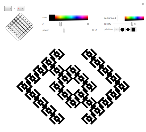
Cha-ching baby. If Snoop Dogg ever used Mathematica, that's what square brackets in his custom font would look like. And I know what this one reminds you of. The folds of the brain. And check out the Black Riddler's Question Mark.

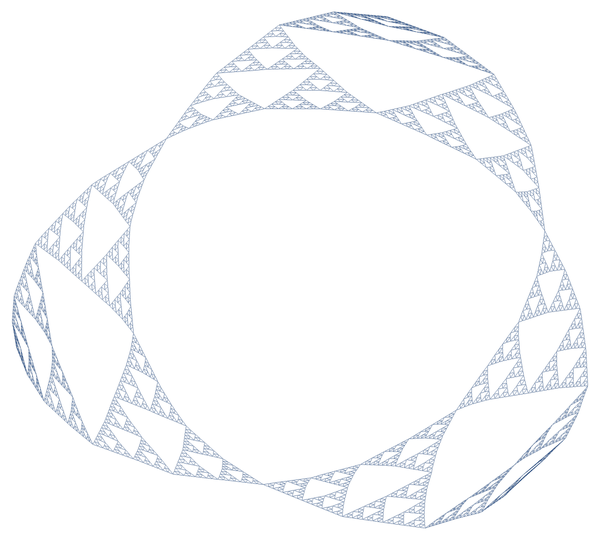
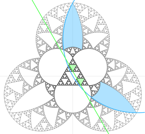
Inversion

axiom = Polygon[{Cos[#], Sin[#]} & /@ (Pi/2 + 2 Pi Range[3]/3)];

next[prev_] := prev /. Polygon[{p1_, p2_, p3_}] :> {
     Polygon[{p1, (p1 + p2)/2, (p1 + p3)/2}],
     Polygon[{p2, (p2 + p3)/2, (p1 + p2)/2}],
     Polygon[{p3, (p1 + p3)/2, (p2 + p3)/2}]};

invert[p_] := p/Norm[p]^2;

draw[n_] := Graphics[{EdgeForm[Black], Nest[next, N@axiom, n]}];

g = draw[2];
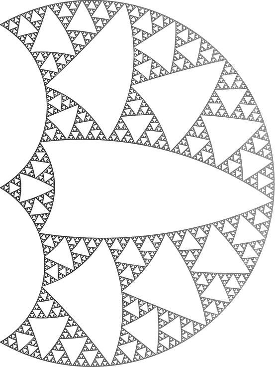
Show[g, g /. Polygon[pts_] :> Polygon[invert /@ pts]]

The radius of inversion is right at the corners of the triangle, and I've left the univerted triangle in the center. Here's what the first few construction steps of the triangle look like if we invert them:

axiom = Polygon[{Cos[#], Sin[#]} & /@ (Pi/2 + 2 Pi Range[3]/3)];

next[prev_] := prev /. Polygon[{p1_, p2_, p3_}] :> {
     Polygon[{p1, (p1 + p2)/2, (p1 + p3)/2}],
     Polygon[{p2, (p2 + p3)/2, (p1 + p2)/2}],
     Polygon[{p3, (p1 + p3)/2, (p2 + p3)/2}]};

invert[p_] := p/Norm[p]^2;

draw[n_] := Module[{ps = Nest[next, N@axiom, n]},
   Graphics[{EdgeForm[Black], Transparent,
     ps, ps /. Polygon[pts_] :> Polygon[invert /@ pts]}]];

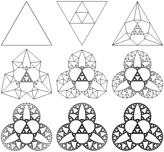
Grid[Partition[draw /@ Range[0, 8], 3]]

Notice that we're just inverting the endpoints of the lines, not the lines-as-curves. Visually this doesn't make a difference at higher iterations:

axiom = Polygon[{Cos[#], Sin[#]} & /@ (Pi/2 + 2 Pi Range[3]/3)];

next[prev_] := prev /. Polygon[{p1_, p2_, p3_}] :> {
     Polygon[{p1, (p1 + p2)/2, (p1 + p3)/2}],
     Polygon[{p2, (p2 + p3)/2, (p1 + p2)/2}],
     Polygon[{p3, (p1 + p3)/2, (p2 + p3)/2}]};

invert[p_] := p/Norm[p]^2;

draw[n_] := Graphics[{
    EdgeForm[Black], Transparent,
    Nest[next, N@axiom, n]}];

Show[draw[10], draw[12] /. Polygon[pts_] :> Polygon[invert /@ pts],
   Method -> {"ShrinkWrap" -> True}, ImageSize -> 4 750] //
  Rasterize // ImageResize[#, Scaled[1/4]] &

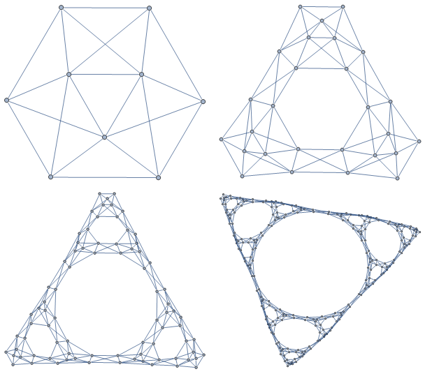
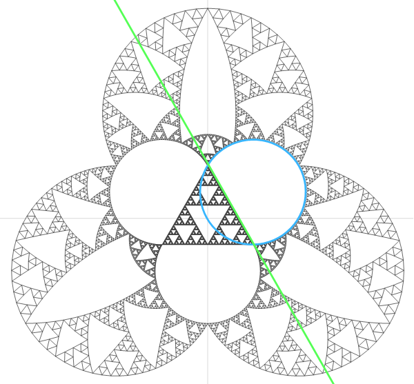
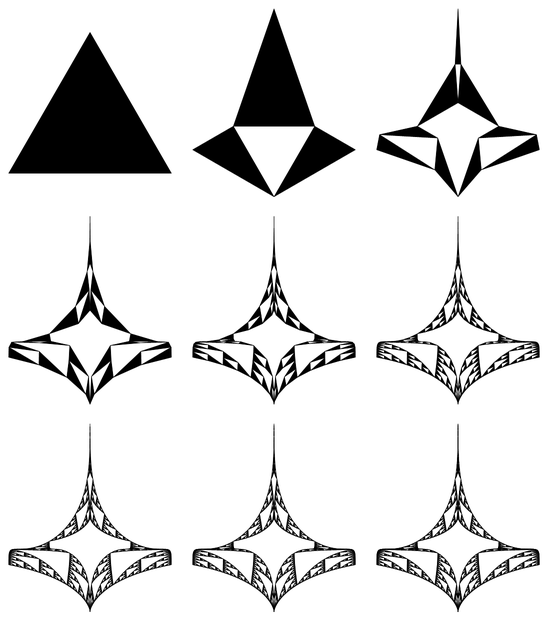
What about varying the radius of inversion? You first perform the same inversion as before, but with respect to the radius:

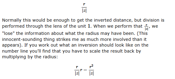
It took me a while, but eventually I realized that the edges of the triangle were being mapped to curves, and that if you continued those curves they would form circles that intersected the origin, like this:

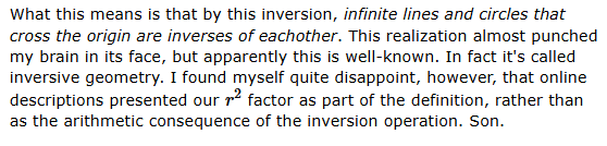
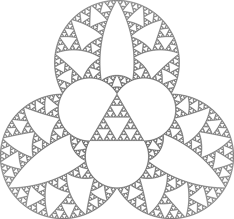
Let's not forget we have a bountiful cornucopia from which to invert:

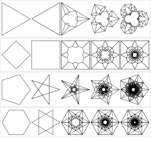
draw[v_, n_] := Module[{ring},
   ring[c_, r_, depth_] := Module[{ps},
     ps = c + r {Cos[#], Sin[#]} & /@ (2 Pi Range[v]/v);

     If[depth == 0, Polygon[ps],
      ring[(c + #)/2, r/2, depth - 1] & /@ ps]];

   Graphics[{Transparent,
     EdgeForm[Black],
     ring[0., 1., n]}]];

Clear[invert];
(*invert[p_/;Norm[p]<.0001]:={0,0};*)
invert[p_] := p/Norm[p]^2;

Column[Panel[Row[#]] & /@
  Table[
   draw[v, n] /. Polygon[pts_] :> Polygon[invert /@ pts],
   {v, 3, 6}, {n, 0, 4}]]

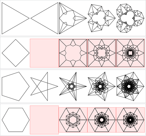
draw[v, n] := Module[{ring}, ring[c, r, depth_] := Module[{ps}, ps = c + r {Cos[#], Sin[#]} & /@ (2 Pi Range[v]/v);

 If[depth == 0, Polygon[ps],
  ring[(c + #)/2, r/2, depth - 1] & /@ ps]];

Graphics[ring[0., 1., n]]];

invert[p_] := p/Norm[p]^2;

Column[Panel[Row[#]] & /@ Table[ draw[v, n] /. Polygon[pts_] :> Line /@ Quiet@Partition[invert /@ pts, 2, 1, 1] /. l_Line /; MemberQ[l, Indeterminate, Infinity] :> {}, {v, 3, 6}, {n, 0, 4}]]

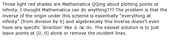
Sidenote. Notice that in this program we aren't even touching our original uninverted geometric renderer, because we don't need to. Our original renderer returns a Graphics structure. This structure (which you might call an M-expression) is to us a set of straightforward vector graphics directives, but is to Mathematica meaningless until the frontend gets ahold of it. Until then (and even afterwards) we can perform the same kinds of structural slicing and dicing that we can perform on any other structure. In this case, replacing points by their inverses.

A more complete solution to our point at infinity/division by 0 problem is to put the inverse of (0, 0) not at infinity, but really far. This doesn't come out of the algebra, but we can do it in a well-behaved way because we know from which direction our lines are coming from since we're defining things as polygons:

invert[p_] := p/Norm[p]^2;

(*you ever see that show Long Ago and Far Away? that show was awesome*)
invertPoly[Polygon[pts_], farAway_: 20000] :=
  With[{indQ = MemberQ[#, Indeterminate] &},
   Line /@ Quiet@Partition[invert /@ pts, 2, 1, 1] /.
    {_?indQ, p_} | {p_, _?indQ} :> {p, farAway Normalize[p]}];

plotRangeInv[g_Graphics] := PlotRange /.
   AbsoluteOptions[g /. Polygon[pts_] :> Quiet@Polygon[invert /@ pts]];

draw[v_, n_] := Module[{ring},
   ring[c_, r_, depth_] := Module[{ps},
     ps = c + r {Cos[#], Sin[#]} & /@ (2 Pi Range[v]/v);

     If[depth == 0, Polygon[ps],
      ring[(c + #)/2, r/2, depth - 1] & /@ ps]];

   Graphics[ring[0., 1., n]]];

(*if it ever came out on DVD i'd buy it like 100 times*)
drawInv[v_, n_] := Module[{g = draw[v, n]},
   Show[g /. poly_Polygon :> invertPoly[poly],
    PlotRange -> 1.1 plotRangeInv[g]]];

(*lines=Cases[drawInv[6,4],Line[ps_]/;
EuclideanDistance@@ps<10000:>Line[Sort[ps]],Infinity];
Graphics[DeleteDuplicates@lines]*)

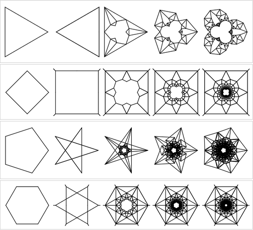
What if, for no particular reason, we vary the exponents of the inversion formula?

axiom = Polygon[{Cos[#], Sin[#]} & /@ (Pi/2 + 2 Pi Range[3]/3)];

next[prev_] := prev /. Polygon[{p1_, p2_, p3_}] :> {
     Polygon[{p1, (p1 + p2)/2, (p1 + p3)/2}],
     Polygon[{p2, (p2 + p3)/2, (p1 + p2)/2}],
     Polygon[{p3, (p1 + p3)/2, (p2 + p3)/2}]};

invert[p_] := p^3/Norm[p]^2;

draw[n_] := Graphics[{EdgeForm[Black],
    Nest[next, N@axiom, n]}];

Grid[Partition[draw /@ Range[0, 8], 3]] /.
 Polygon[pts_] :> Polygon[invert /@ pts]

See this one. One day you're going to be driving home from work. It's going to be dark. Pitch black. All a sudden out the corner your eye you're gonna see a flash in your rear view mirror. And when you look, you're gonna see that same Black Cobra Grill on my car speeding towards you at some unspeakable number of kilometers per hour. And then I'll disappear into the night. Like an episode off an MJ's Thriller×Knight Rider mashup.

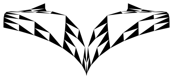
If we mangle the formula every which way we can find a lot of interesting effects:

axiom = Polygon[{Cos[#], Sin[#]} & /@ (Pi/4 + 2 Pi Range[3]/3)];

next[prev_] := prev /. Polygon[{p1_, p2_, p3_}] :> {
     Polygon[{p1, (p1 + p2)/2, (p1 + p3)/2}],
     Polygon[{p2, (p2 + p3)/2, (p1 + p2)/2}],
     Polygon[{p3, (p1 + p3)/2, (p2 + p3)/2}]};

transform[p_] := (Reverse[p].p) p^2/Norm[p]^2;

drawFishie1[n_] := Graphics[{Red,
    EdgeForm[{Thickness[.01], Opacity[.3],
      JoinForm["Round"], Lighter[Blue, .6]}],
    Rotate[Nest[next, N@axiom, n] /.
      Polygon[pts_] :> Polygon[transform /@ pts], 3 Pi/4]},
   PlotRange -> .8 {{-.85, 1.51}, .4 {-1, 1.1}}];

drawFishie2[n_] := Graphics[{
    Transparent, EdgeForm[Black],
    Rotate[Nest[next, N@axiom, n] /.
      Polygon[pts_] :> Polygon[transform /@ pts], -Pi/4]}];

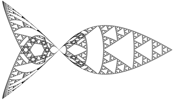
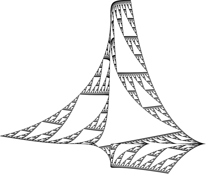
The self-crossings form hexagonal figures. And American iconography? Here's another nifty one:

next[prev_] := prev /. Polygon[{p1_, p2_, p3_}] :> {
     Polygon[{p1, (p1 + p2)/2, (p1 + p3)/2}],
     Polygon[{p2, (p2 + p3)/2, (p1 + p2)/2}],
     Polygon[{p3, (p1 + p3)/2, (p2 + p3)/2}]};

transform[p_] := (Reverse[p].p) p/Norm[p]^2;

notFishieAwwwSadFace[n_, a1_: 0, a2_: 0, options___] :=
  Module[{axiom},
   axiom = Polygon[{Cos[#], Sin[#]} & /@ (a1 + 2 Pi Range[3]/3)];

   Graphics[{Transparent, EdgeForm[Black],
     Rotate[Nest[next, N@axiom, n] /.
       Polygon[pts_] :> Polygon[transform /@ pts], a2]},
    options]];

notFishieAwwwSadFace[6, Pi/4]

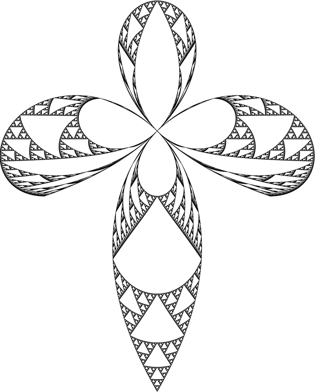
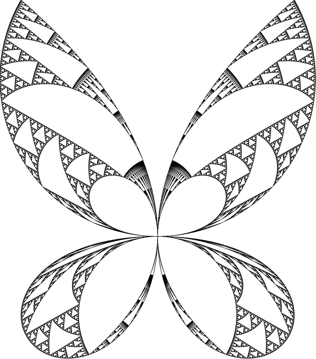
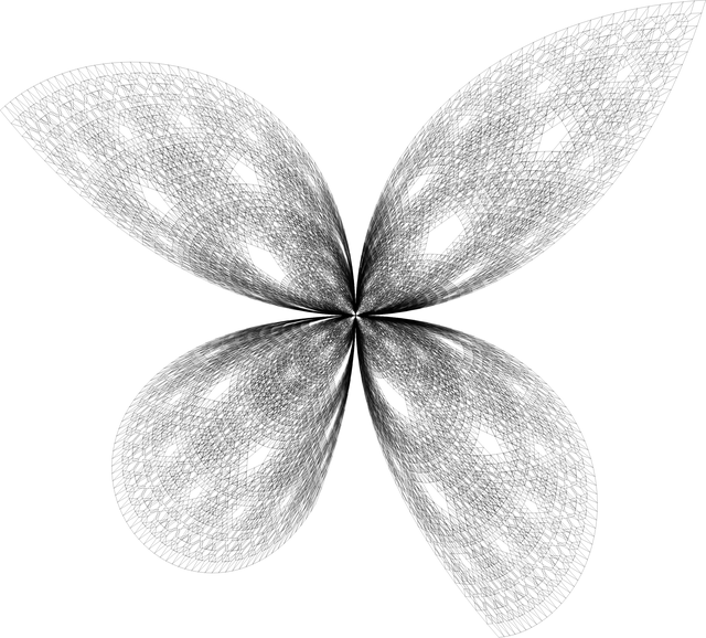
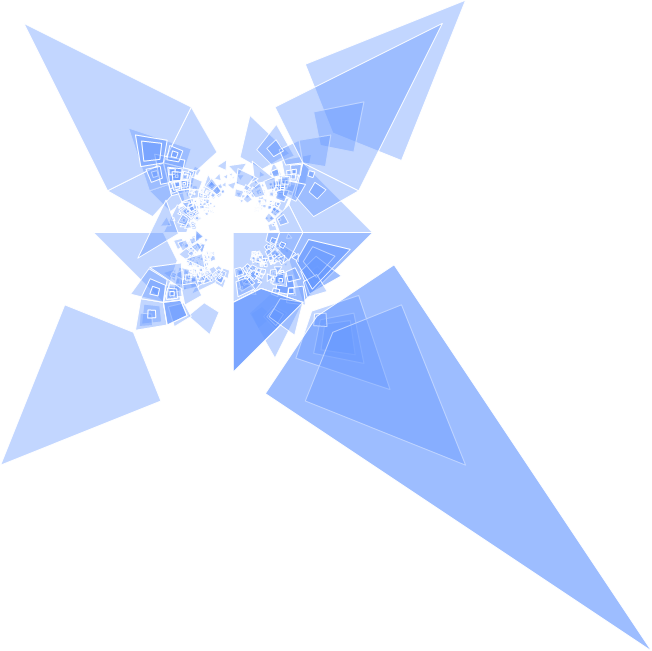
I call it the Sierpinski Stiletto of Triangular Destruction. Hell yea. Also pay heed to the Sierpinski Butterfly of Poisonous Death, lest yee regret it. We can also move the circle of inversion around. I was going to write a program to do only that, but before I realized it I had accidentally built this:

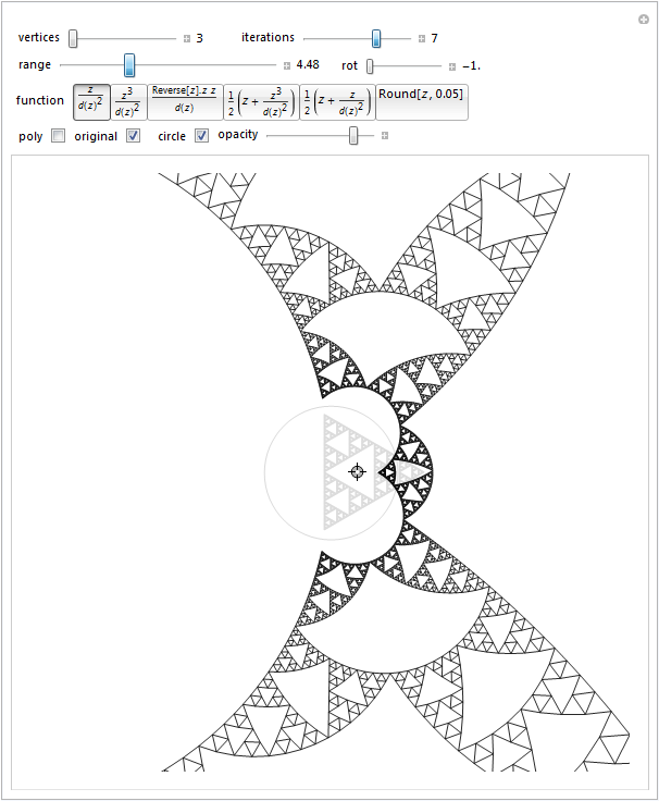
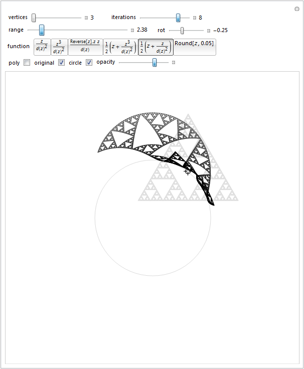
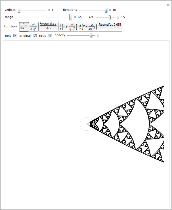
polys[v_, n_, offset_: {0, 0}, size_: 1, rot_: 0] := Module[{ring},
   ring[c_, r_, depth_] := Module[{ps},
     ps = c + r {Cos[#], Sin[#]} & /@ (rot + 2 Pi Range[v]/v);

     If[depth == 0, Polygon[(offset + # &) /@ ps],
      ring[(c + #)/2, r/2, depth - 1] & /@ ps]];

   ring[0., size, n]];

(*Polygon in, Lines out /statictyping*)
invertPoly[Polygon[pts_], tf_, farAway_: 20000] :=
  With[{indQ = MemberQ[#, Indeterminate] &},
   Line /@ Quiet@Partition[tf /@ pts, 2, 1, 1] /.
    {_?indQ, p_} | {p_, _?indQ} :> {p, farAway Normalize[p]}];

d = Norm;
(*d=ChessboardDistance[{0, 0},#]&;*)
transformationFunctions = {
   #/d[#]^2 &,
   #^3/d[#]^2 &,
   (Reverse[#].#) #/d[#] &,
   (# + #^3/d[#]^2)/2 &,
   (# + #/d[#]^2)/2 &,
   Round[#, .05] &};

With[{
  verticesC = Control[{{vertices, 3}, 3, 8, 1, Appearance -> "Labeled", ImageSize -> Small}],
  iterationsC = Control[{{iterations, 5}, 0, 10, 1, Appearance -> "Labeled", ImageSize -> Small}],
  rangeC = Control[{{range, 4}, 1, 12, Appearance -> "Labeled"}],
  rotC = Control[{{rot, -Pi/6}, -Pi, Pi, Appearance -> "Labeled", ImageSize -> Tiny}],
  functionC = {{tf, transformationFunctions[[1]], "function"},
    (# -> TraditionalForm@Quiet@Trace[#[z]][[2]] &) /@ transformationFunctions,
       ControlType -> SetterBar},
  originalC = Control[{original, {True, False}}],
  circleC = Control[{circle, {True, False}}],
  opacityC = Control[{{opacity, 1}, 0, 1, ImageSize -> Small}],
  sizeC = Control[{{size, 1}, .001, 4, ImageSize -> Small}],
  offsetC = {{offset, {0, 0}}, Locator}},

 Manipulate[Module[{polygons},
   polygons = polys[vertices,
     ControlActive[Min[3, iterations - 2], iterations],
     offset, size, rot];

   Graphics[{
     If[circle, {LightGray, Circle[]}],
     If[original, {EdgeForm[LightGray], {Transparent, polygons}}],
     {Black, polygons /. p_Polygon :> invertPoly[p, tf]}},
    PlotRange -> range]],

  Row[{verticesC, iterationsC}],
  Row[{rangeC, rotC}], functionC,
  Row[{originalC, circleC, sizeC, opacityC}, "  "], offsetC,
  SynchronousUpdating -> False]]

Oops. This hilarious function doesn't allow anything inside the unit disk. It's just waiting for someone to make a Yakety Sax movie about shapes crashing into the circle and crawling around it.

Someone on the internet asked an interesting question: Are there "zoom out" fractals? We know that if we zoom in on the Sierpinski triangle, we'll continue seeing detail endlessly. But are there fractals that no matter how far you zoom out, you can't get out of them?

Of course there are. We can just take a quote-unquote "zoom in" fractal and place one of its points of detail right at the origin, and then invert the fractal. Because the inverse of the origin is some kind of crazy infinity, we know that no matter how far we zoom out, we won't reach the end of the fractal. This example is really a formality though. You have a lot of liberty to make things up in math.

Cornucopia.

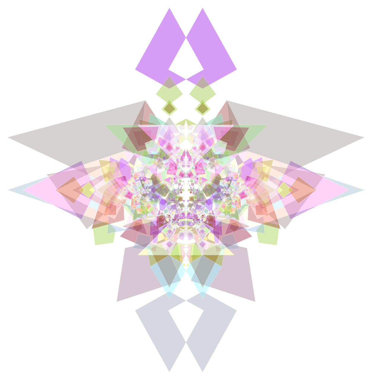
invert[p_ /; Norm[p] < .0001] := {0, 0};
invert[p_] := p/Norm[p]^2;

draw[v_, df_, n_] := Module[{ring},
   ring[c_, r_, depth_] := Module[{ps},
     ps = c + r {Cos[#], Sin[#]} & /@ (2. Pi Range[v]/v);

     If[depth == 0, Polygon[invert /@ ps],
      ring[(c + #)/2, df[0, r], depth - 1] & /@ ps]];

   Graphics[{EdgeForm[White], Opacity[.4],
     RGBColor[.4, 1(*;.6*), 1], ring[0., 1., n]}]];

candy[g_, res_: 600, upsc_: 1, style_: EdgeForm[Thick]] :=
  Module[{a = Show[g, ImageSize -> upsc res, Background -> White]},

   a = a /. p_Polygon :>
      {RGBColor[.6, RandomReal[], RandomReal[]], style, p};
   a = Rasterize[a];

   (*move this downscale to end for different quality*)
   a = ImageResize[a, Scaled[1/upsc]];
   ImageDifference[a, ImageReflect[a, Left]] // ColorNegate];

g = With[{f = (#1 + #2)/RandomChoice[Prime[Range[4]]] &},
  Show[
   Table[draw[(*repeatedly draw to cover more possibilities*)
      RandomChoice[{1, 1, .25} -> {3, 4, 5}], f,
      RandomChoice[{.1, 1.5} -> {2, 3}]]
     /. p_Polygon :> Rotate[p, 0(*;Pi/4*), {0, 0}],
    {12}], Background -> Black, ImageSize -> Medium]];

(*note you can edit g in-place*)
Defer[candy][g, 1280, 4]

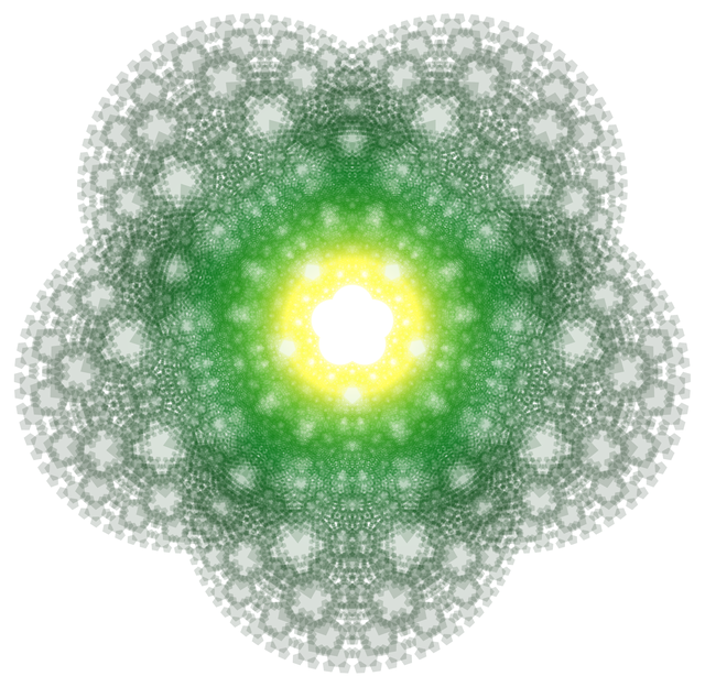
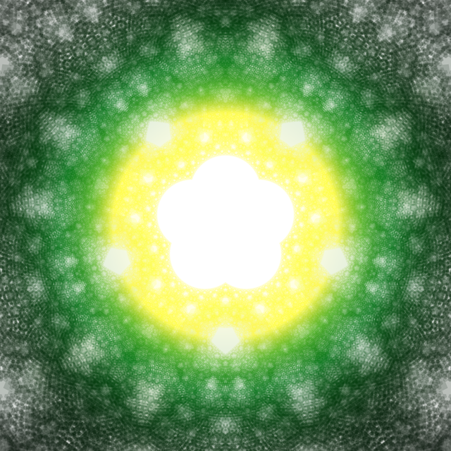
ring[c_, r_, depth_] := Module[{ps},
   ps = c + r {Cos[#], Sin[#]} & /@ (-Pi/10 + 2. Pi Range[5]/5);

   If[depth == 0, Polygon[ps],
    ring[#, r/2, depth - 1] & /@ ps]];

invert[p_] := p/Norm[p]^2;

Graphics[{Opacity[.15], Black,
   ring[0., 1., #] & /@ Range[5(*;8*)]}] /.
 Polygon[pts_] :> Polygon[invert /@ pts, VertexColors ->
   (ColorData["AvocadoColors"] /@ (#^1.7 &) /@ Norm /@ pts)]

From what I can tell, one of the settings used to deal with division by 0 is the so-called Riemann sphere, which is where we take a space shuttle and use it to fly over and drop a cow on top of a biodome, and then have the cow indiscriminately fire laser beams at the grass inside and around the biodome. That's my intuitive understanding of it anyway.

shuttle = ExampleData[{"Geometry3D", "SpaceShuttle"}, "GraphicsComplex"];
cow = ExampleData[{"Geometry3D", "Cow"}, "GraphicsComplex"];
grass = ExampleData[{"Texture", "Grass4"}];
drop = Sound[Play[Sin[1000 (2 - t)^2.3], {t, 0, .9}]];
lazer[] := EmitSound[Sound[Play[{TriangleWave[10 (2 - t)^5],
      Sin[500 (2 - t)^5] + SawtoothWave[20 (2 - t)^4.99]},
     {t, 0, .2}, SampleRate -> 4000]]];

Animate[Module[{dir, angle},
  (*xs animates from +30 to -60*)
  If[xs > 25, dropTrigger = False];
  If[dropTrigger == False && xs < 10, dropTrigger = True; EmitSound[drop]];
  If[xs < -10,
   lazer[];
   dir = RandomReal[{-15, 15}, 2]~Join~{-20};
   angle = ArcTan @@ Take[dir, 2], angle = 0];

  Labeled[#, Style["Understanding the Riemann Sphere", FontFamily -> "Verdana"], Top] &@
   With[{
     cowLoc = {Clip[xs, {1.3, 50}], 0, Clip[8 + (-(.25 xs - 5)^2), {-13, -.25}]},
     greenLight = Lighting -> {{"Directional", Green, {{5, 5, 5}, {0, 0, 0}}}}},

    Graphics3D[{EdgeForm[None],
      (*shuttle*){Specularity[White, 7], Translate[shuttle, {xs, 0, 0}]},
      (*cow*) Rotate[Translate[Scale[cow, 5], cowLoc], angle, {0, 0, 1}],

      (*grass*) Translate[{If[False, Sequence @@ {greenLight, Texture[grass]}, Green],
        Polygon[50 {{-1, -1, 0}, {1, -1, 0}, {1, 1, 0}, {-1, 1, 0}},
         VertexTextureCoordinates -> 1.1 {{0, 0, 0}, {1, 0, 0}, {1, 1, 0}, {0, 1, 0}}]},
        {0, 0, -19}],

      (*biodome*){Specularity[White, 3], Opacity[.5], Sphere[.95 {0, 0, -20}, 5]},
      (*sun*){Glow[White], Sphere[{18, 18, 18}, 2]},
      (*laser*) If[xs < -10, {Red, Glow[Red], Opacity[.5], Tube[{{0, 0, -12.4}, dir}]}]},
     (*sky*)Background -> LightBlue, PlotRange -> 20, Boxed -> False]]],
 {xs, 30, -60, 3.2}, AnimationRate -> 10, DisplayAllSteps -> True]

(Note the cow cannot be spherical or it will roll off). Personally I don't have any beef with Riemann or any of his manifolds, but for our purposes the Riemann sphere is inadequate since it maps our inverses vertically. One interesting consequence of this is that in the 2D cross section where the imaginary component is zero (essentially the 'Weierstrass circle'), it maps multiplicative inverses vertically and additive inverses horizontally. This all seems mathematically expedient, but it's otherwise boring.

The Riemann sphere does give one explanation though about 'why' our circles and lines are inverses. In the Riemann sphere, the inverse of a circle that crosses the origin is a circle that crosses the North Pole, and since the lasers are being shot from the North Pole, they're limited to tracing out a line as they follow the circle. I was going to make a simple 3D diagram demonstrating this, but I accidentally made this:

toRiemann = Compile[{{pts, _Real, 2}}, Module[{k},
    Map[(k = 2/(1 + #.#);
       {k #[[1]], k #[[2]], 1 - k}) &, pts]]];

fromRiemann[pts_] := (-1/(#3 - 1)) {#1, #2, 0} & @@@ pts;

shuttle = ExampleData[{"Geometry3D", "SpaceShuttle"}, "GraphicsComplex"];
cow = Append[ExampleData[{"Geometry3D", "Cow"}, "GraphicsComplex"],
   VertexTextureCoordinates -> 1/500 ExampleData[{"Geometry3D", "Cow"}, "PolygonData"]];
sphere = SphericalPlot3D[1, {\[Theta], 0, Pi}, {\[Phi], 0, 2 Pi},
   MeshStyle -> Opacity[.05], PlotStyle -> Opacity[.1]];
plane = {Lighting -> "Neutral", Opacity[.5], LightGray, EdgeForm[None],
   Line[{{-50, 0, 0}, {50, 0, 0}}], Line[{{0, -50, 0}, {0, 50, 0}}],
   Polygon[15 {{-1, -1, 0}, {1, -1, 0}, {1, 1, 0}, {-1, 1, 0}}]};

numPoints = 160/4;
circle = .25 {1 + Cos[#], Sin[#], 0} & /@ (-Pi + 2 Pi Range[numPoints]/numPoints);
rCircle = toRiemann[circle];
invRCircle = {#1, #2, -#3} & @@@ rCircle;
invCircle = Quiet[fromRiemann[invRCircle]];

ind = Indeterminate {1, 1, 1};
transform[\[Theta]_] := Composition[
   RotationTransform[\[Theta], {0, 0, 1}],
   TranslationTransform[{0, 0, 1.2}]];
{l, r} = {{.335, -.044, .1894}, {.335, .044, .1894}};

slides = ParallelTable[Module[{angle},
    angle = Quiet[ArcTan @@ (invCircle /. ind -> {0, 0})[[pti, 1 ;; 2]] /.  ArcTan[0, 0] -> 0];
    Show[sphere,
     Graphics3D[{
       plane, Opacity[.7], Sphere[{0, 0, 1}, .01],
       (*cow*) Rotate[#, angle, {0, 0, 1}] &@Translate[#, {0, 0, 1.2}] &@
        {EdgeForm[None],(*Opacity[.999],*)Texture[Graphics[Disk[]]],
         Lighting -> "Neutral", Lighting -> {{"Point", Darker[Red], l}},
         cow, Red, Glow[Red], Sphere[{l, r}, .01]},
       (* keep shuttle in orbit in case need more cows *)
       {EdgeForm[None], Translate[shuttle, {0, 0, 100}]},
       (*lazerz*) If[invCircle[[pti]] =!= ind, {Red,
         Line[{transform[angle][l], invCircle[[pti]]}],
         Line[{transform[angle][r], invCircle[[pti]]}],
         {Red, Glow[Red], Opacity[.1], Sphere[invCircle[[pti]], .02 RandomReal[]]}}],
       (*etc*) {Lighter[Gray], Dashed, Line[{rCircle[[pti]], invRCircle[[pti]]}]},
       {Opacity[.1], Lighter[Blue], Line[circle]},
       {Opacity[.5], Lighter[Blue], Line[Take[circle, pti]]},
       {Lighter[Blue], Line[{{0, 0, 1}, 50 (-{0, 0, 1} + circle[[pti]])}]},
       {Lighter[Blue], Line[Take[rCircle, pti]]},
       {Red, Line[Take[invRCircle, pti]]},
       (*Purple,Line[{{0,0,1},50(-{0,0,1}+invCircle[[pti]])}/.tride->{0,0,1}],*)
       (*burn mark*) Thick, Red, Line[DeleteCases[Take[invCircle, pti], ind]]}],
     ImageSize -> 1/4 {16, 9} (1080/9),
     ViewAngle -> 4 Degree, PlotRange -> 10, Boxed -> False, Axes -> False]],
   {pti, 1, Length[circle]}];
ListAnimate[slides]

Oops. But since we now have this tool, let's see what other plots look like:

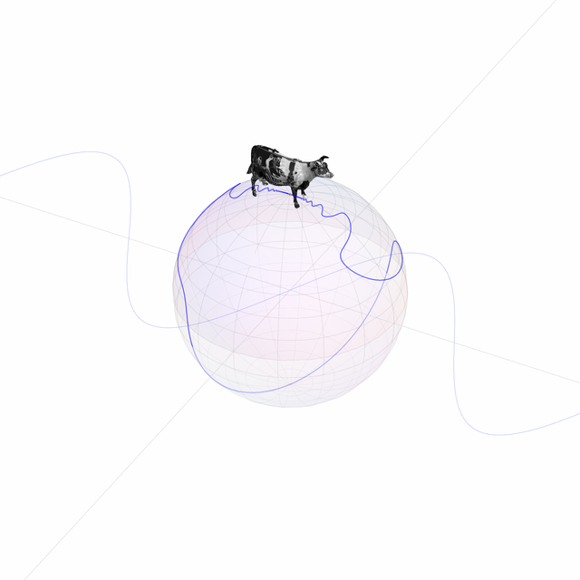
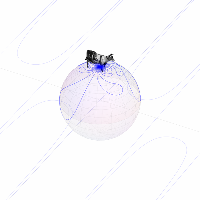
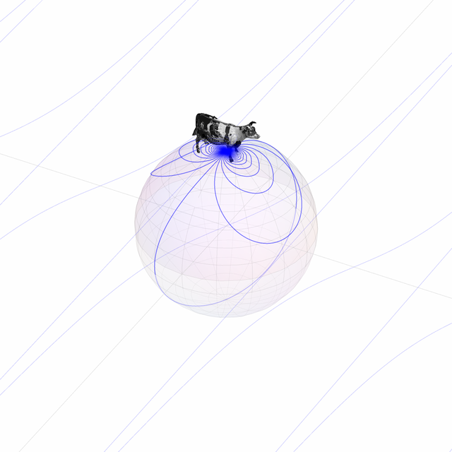
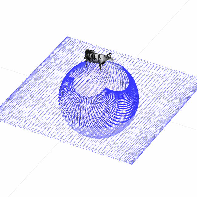
toRiemann = Compile[{{pts, _Real, 2}}, Module[{k},
    Map[(k = 2/(1 + #.#);
       {k #[[1]], k #[[2]], 1 - k}) &, pts]]];

shuttle = ExampleData[{"Geometry3D", "SpaceShuttle"}, "GraphicsComplex"];
cow = Append[ExampleData[{"Geometry3D", "Cow"}, "GraphicsComplex"],
   VertexTextureCoordinates -> 1/500 ExampleData[{"Geometry3D", "Cow"}, "PolygonData"]];
sphere = SphericalPlot3D[1, {\[Theta], 0, Pi}, {\[Phi], 0, 2 Pi},
   MeshStyle -> Opacity[.05], PlotStyle -> Opacity[.1]];
plane = {Lighting -> "Neutral", Opacity[.5], LightGray, EdgeForm[None],
   Line[{{-50, 0, 0}, {50, 0, 0}}], Line[{{0, -50, 0}, {0, 50, 0}}],
   Polygon[15 {{-1, -1, 0}, {1, -1, 0}, {1, 1, 0}, {-1, 1, 0}}]};

listRiemannPlot[pts_] := Module[{rPts = toRiemann[pts]},
   Show[
    sphere,
    Graphics3D[{
      plane, Opacity[.7], Sphere[{0, 0, 1}, .01],

      (*cow*)Translate[#, {0, 0, 1.2}] &@
       {EdgeForm[None],(*Opacity[.999],*)
        Texture[Graphics[Disk[]]], Lighting -> "Neutral", cow},

      (*shuttle*){EdgeForm[None], Translate[shuttle, {0, 0, 100}]},
      (*original*){Opacity[2 .2], Lighter[Blue], Line[pts]},
      (*riemannized*){Opacity[.8], Blue, Line[rPts]}}],

    ViewAngle -> 4 Degree, PlotRange -> 10, Boxed -> False, Axes -> False]];

listRiemannPlot[Table[{x, Sin[2 x], 0}, {x, -40 Pi, 40 Pi, .01}]]

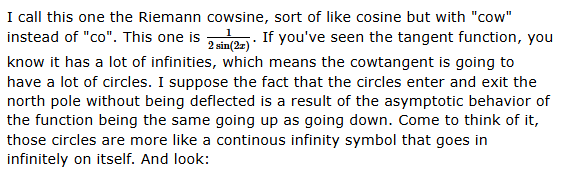
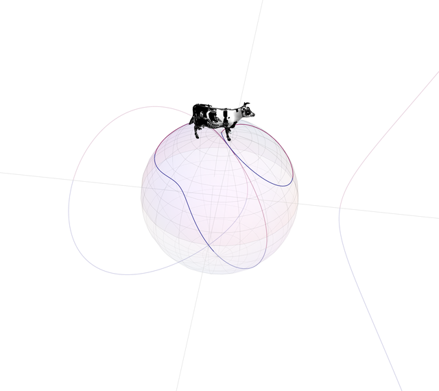
toRiemann = Compile[{{pts, _Real, 2}}, Module[{k},
    Map[(k = 2/(1 + #.#);
       {k #[[1]], k #[[2]], 1 - k}) &, pts]]];

shuttle = ExampleData[{"Geometry3D", "SpaceShuttle"}, "GraphicsComplex"];
cow = Append[ExampleData[{"Geometry3D", "Cow"}, "GraphicsComplex"],
   VertexTextureCoordinates -> 1/500 ExampleData[{"Geometry3D", "Cow"}, "PolygonData"]];
sphere = SphericalPlot3D[1, {\[Theta], 0, Pi}, {\[Phi], 0, 2 Pi},
   MeshStyle -> Opacity[.05], PlotStyle -> Opacity[.1]];
plane = {Lighting -> "Neutral", Opacity[.5], LightGray, EdgeForm[None],
   Line[{{-50, 0, 0}, {50, 0, 0}}], Line[{{0, -50, 0}, {0, 50, 0}}],
   Polygon[15 {{-1, -1, 0}, {1, -1, 0}, {1, 1, 0}, {-1, 1, 0}}]};

riemannize[Graphics[g_, rest___], options___] :=
  Show[sphere,
   Graphics3D[{plane,
     (*cow*)Translate[#, {0, 0, 1.2}] &@
      {EdgeForm[None],
       Texture[Graphics[Disk[]]], Lighting -> "Neutral", cow},
     (*shuttle*)Translate[shuttle, {0, 0, 100}],
     (*curves*)g /. Line[pts_] :> {Line[toRiemann[pts]],
        Opacity[.25], Line[{#1, #2, 0} & @@@ pts]}}],
   Boxed -> False, Axes -> None, PlotRange -> 5, options];

plot = Plot[
   Evaluate[y /. Solve[y^2 == x^3 - 3 x + 1, y]],
   {x, -100, 100}, PlotPoints -> 10000];

riemannize[plot, ViewAngle -> 15 Degree]

This is one of those fangled elliptic curves. Apparently they do form pairs of circle things on the Riemann sphere. I thought that was just an old wive's tale. The nice thing about this program is that it works on Graphics structures, such as those returned by Plot. That means you can plug arbitrary 2D plots and graphics into this function and have them automatically Riemannized. Like say you're trying to educe from without your incorrigible students' crania some particular factoid:

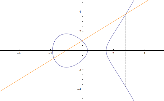
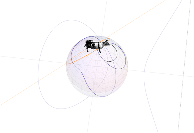
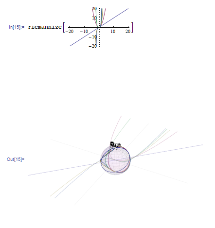
toRiemann = Compile[{{pts, _Real, 2}}, Module[{k},
    Map[(k = 2/(1 + #.#); {k #[[1]], k #[[2]], 1 - k}) &, pts]]];

shuttle = ExampleData[{"Geometry3D", "SpaceShuttle"}, "GraphicsComplex"];
cow = Append[ExampleData[{"Geometry3D", "Cow"}, "GraphicsComplex"],
   VertexTextureCoordinates -> 1/500 ExampleData[{"Geometry3D", "Cow"}, "PolygonData"]];
sphere = SphericalPlot3D[1, {\[Theta], 0, Pi}, {\[Phi], 0, 2 Pi},
   MeshStyle -> Opacity[.05], PlotStyle -> Opacity[.1]];
plane = {Lighting -> "Neutral", Opacity[.5], LightGray, EdgeForm[None],
   Line[{{-50, 0, 0}, {50, 0, 0}}], Line[{{0, -50, 0}, {0, 50, 0}}],
   Polygon[15 {{-1, -1, 0}, {1, -1, 0}, {1, 1, 0}, {-1, 1, 0}}]};

riemannize[Graphics[g_, ___], options___] := Show[sphere,
   Graphics3D[{plane,
     (*cow*)Translate[#, {0, 0, 1.2}] &@
      {EdgeForm[None],(*Opacity[.999],*)
       Texture[Graphics[Disk[]]], Lighting -> "Neutral", cow},
     (*shuttle*)Translate[shuttle, {0, 0, 100}],
     (*curves*)g /. Line[pts_] :> {Line[toRiemann[pts]],
        Opacity[.25], Line[{#1, #2, 0} & @@@ pts]}}],
   Boxed -> False, Axes -> None, PlotRange -> 5, options];

vint = Sqrt[1 - 3/2 (1 + Sqrt[21]) + 1/8 (1 + Sqrt[21])^3];
plot = Show[Plot[y /. Solve[y^2 == x^3 - 3 x + 1, y], {x, -100, 100}, PlotPoints -> 10000],
   Graphics[{Orange, Line[Table[{x, x + 1}, {x, -500, 500, .1}]],
     Black, Dashing[1/10 {0.08, 0.02}],
     Line[Table[{1/2 (1 + Sqrt[21]), y}, {y, -vint, vint, .1}]]}]];

riemannize[plot, ViewAngle -> 8 Degree]

You've set this up with 2D graphics. But you can just plug the output of this into our Riemannizer to get this. In fact in Mathematica you can even copy/paste the 2D plot (itself an interactwithable vector object) like this. And you can vector-edit that plot in-place and when you re-evaluate the expression, the differences will appear in the Riemannization. Not bad for what essentially amounts to one line of code:

g /. Line[pts_] :> Line[toRiemann[pts]]

This is the power of Mathematica's macro-at-will symbolic semantics and well-curated architecture. Specifically in this case, it's the fact that the built-in plotting functions return the same laid-bare Graphics vector structures that your own versions of those functions would return. This Riemannizer only does a direct endpoint conversion of lines, but you can easily have it 3Dify whatever you want in a more thorough fashion.

After I made my Cyclotron 4000 masterpiece, I considered what a version 2 might be. Now I know. With some adjustments to the contraption, we now have the Cycowtron 4800 Deluxe (pronounced psy-cow-tron forty-eight-hundred de-lux):

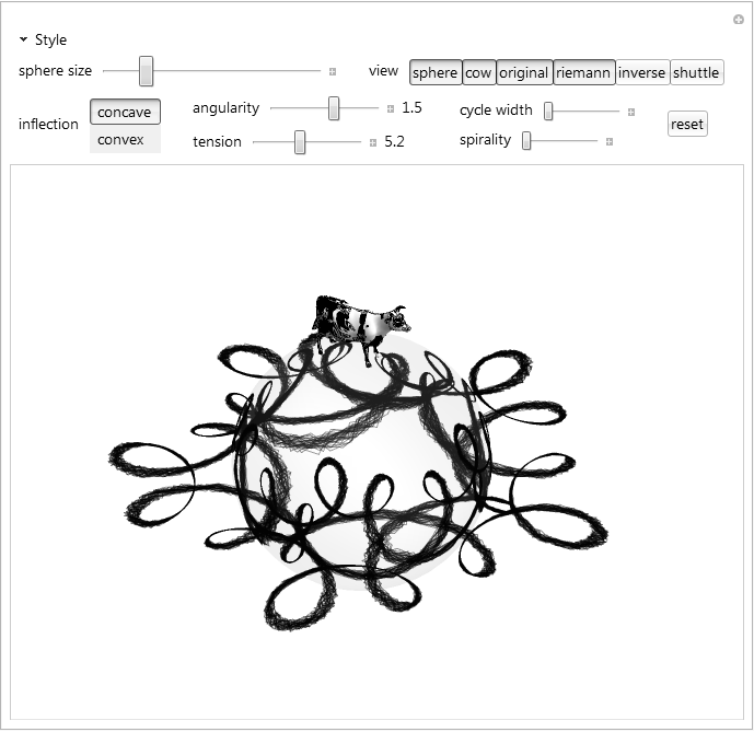
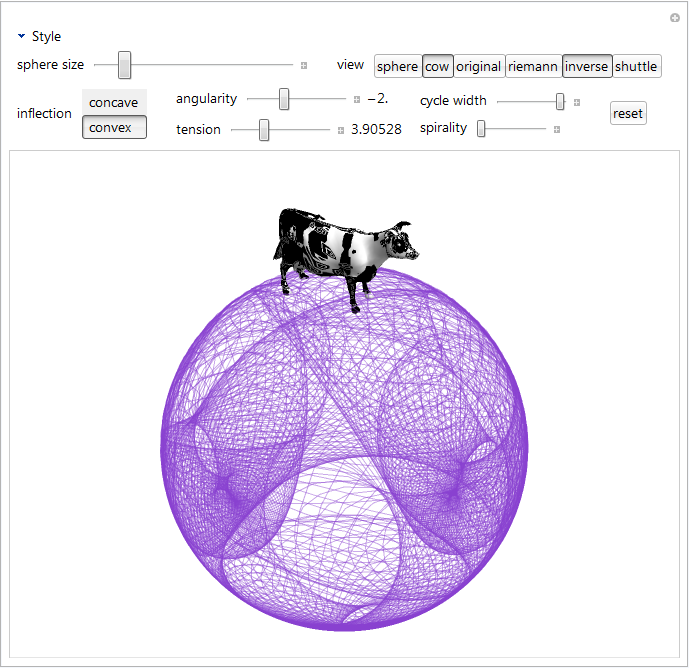
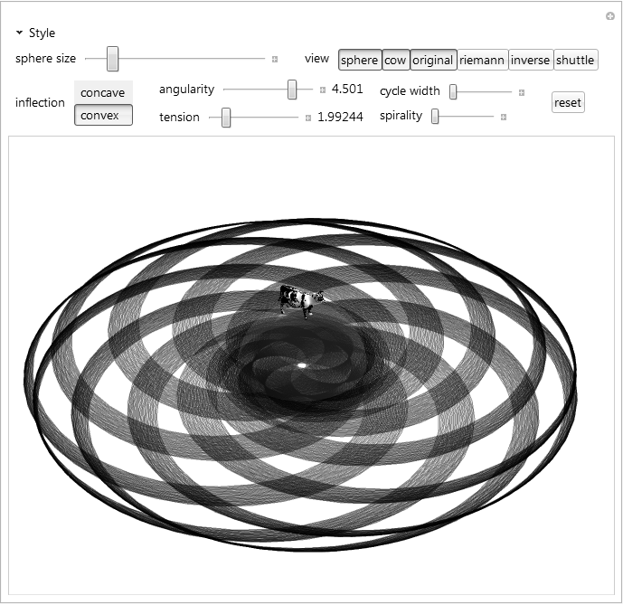
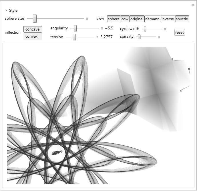
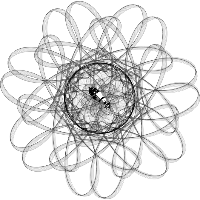
toRiemann = Compile[{{pts, _Real, 2}}, Module[{k},
    Map[(k = 2/(1 + #.#); {k #[[1]], k #[[2]], 1 - k}) &, pts]]];

invertRiemann[pts_] := {#1, #2, -#3} & @@@ pts;
(*fromRiemann[pts_]:=(-1/(#3-1)) {#1,#2,0}&@@@pts;*)

shuttle = With[{shuttleGC = ExampleData[{"Geometry3D", "SpaceShuttle"}, "GraphicsComplex"]},
   Translate[#, {0, 0, 100}] &@
    {EdgeForm[None], Lighting -> "Neutral",
     Append[shuttleGC, VertexColors -> RandomReal[.65 + {0, 1}, Length[shuttleGC[[1]]]]^2]}];

cow = Translate[#, {0, 0, 1.2}] &@
   {EdgeForm[None],(*Opacity[.999],*)Texture[Graphics[Disk[]]], Lighting -> "Neutral",
    Append[ExampleData[{"Geometry3D", "Cow"}, "GraphicsComplex"],
     VertexTextureCoordinates -> 1/500 ExampleData[{"Geometry3D", "Cow"}, "PolygonData"]]};

allSettings = {"sphere", "cow", "original", "riemann", "inverse", "shuttle"};

bookmarks = {
   "Random" :> (
     With[{R := RandomReal[]},
      color = RGBColor[R, R, R];
      inflection = RandomChoice[{1, -1}];
      effect = .25*R^8; thickness = 10*R^8;
      spirality = R^3;
      If[spirality < .035, spirality = 0];
      x = 12 R; y = 2 R];

     Module[{weights = If[x > 3, {.1, .03, .87}, {.1, .07, .83}]},
      \[Zeta] = RandomChoice[{-1, 1}]*
        RandomChoice[weights -> {
           RandomReal[{0, 7.5}],
           RandomChoice[{0, .5, .5}],
           Round[RandomReal[{1, 7.5}], .5]}]]),

   "Rose" :> {color = Red, effect = 0, inflection = -1, x = 0, y = 1.1343, spirality = 0, \[Zeta] = 3},
   "Glyph" :> {color = Black, effect = 0.198, inflection = 1, x = 5.2, y = 0, spirality = 0, \[Zeta] = 2},
   "Mass Atomic" :> { effect = 0, inflection = -1, x = 5.84, y = 0.412, spirality = 0, \[Zeta] = -4.2504},
   "Jello" :> {color = Red, effect = 0, inflection = -1, x = 12, y = 0.846, spirality = 1, \[Zeta] = -1},
   "Grim" :> {thickness = 3.35, color = Black, effect = 0.0675, inflection = 1, x = 8, y = 0.296, spirality = 1, \[Zeta] = -1},
   "Angelwings" :> {color = RGBColor[.07694, .39046, 1], effect = 0, inflection = 1, spirality = 1, x = 12, y = 0, \[Zeta] = -5.4947},
   "Rollers" :> {color = Black, effect = 0, inflection = -1, spiral3ity = 0, x = 5.5, y = .1, \[Zeta] = -0.984032039033508},
   "Lifespark" :> {color = RGBColor[.1026, .9878, .0201], effect = 0, inflection = 1, spirality = .0995, x = 3.2757, y = .2002, \[Zeta] = -5.5}};

With[{
  colorC = Control[{{color, Black, "line color"}, ColorSlider}],
  backgroundC = Control[{{background, White}, ColorSlider}],
  thicknessC = Control[{{thickness, .001, "line thickness"}, .001, 10, Appearance -> "Labeled", ImageSize -> Small}],
  effectC = Control[{{effect, 0., "charcoal effect"}, 0, .25, Appearance -> "Labeled", ImageSize -> Small}],
  inflectionC = Control[{{inflection, 1}, {1 -> " concave ", -1 -> " convex "}, Appearance -> "Vertical"}],
  angularityC = Control[{{\[Zeta], 2., "angularity"}, -7.5, 7.5, .5, Appearance -> "Labeled", ImageSize -> Small}],
  tensionC = Control[{{x, 8., "tension"}, 0, 12, Appearance -> "Labeled", ImageSize -> Small}],
  yC = Control[{{y, 2., "cycle width"}, 0, 2, ImageSize -> Tiny}],
  spiralityC = Control[{{spirality, 0.}, 0, 1, ImageSize -> Tiny}],
  scaleC = Control[{{scale, 3.157, "sphere size"}, .00001, 15, ImageSize -> Medium}],
  settingsC = Control[{{settings, Take[allSettings, 4], "view"}, allSettings, ControlType -> TogglerBar}],
  opacityC = Control[{{opacity, .43}, 0, 1, Appearance -> "Labeled", ImageSize -> Small}],
  resetC = DynamicWrapper[
    Tooltip[Setter[Dynamic[reset], "reset"], "reset perspective", TooltipDelay -> .3],
    If[reset === "reset", (reset = False; vp = {1.3, -2.4, 2}; vv = {0, 0, 1}; {va, vc} = Automatic {1, 1})]]},

 With[{
   controls = Sequence[
     OpenerView[{"Style",
       Column[{
         Row[{
           Column[{backgroundC, colorC}, Alignment -> Right],
           Column[{effectC, thicknessC, opacityC}, Alignment -> Right]},
          Spacer[30]],
         Style[\[HorizontalLine], Lighter[LightGray]]}, Spacings -> 0]}],
     Row[{scaleC, Spacer[30], settingsC}],
     Row[{inflectionC, Spacer[30],
       Column[{angularityC, tensionC}],
       Column[{yC, spiralityC}], Spacer[30], resetC}]],

   storedVars = Sequence @@ ({{#, Automatic}, ControlType -> None} & /@ {vp, vv, va, vc}),
   dynamicView = Sequence[
     ViewPoint -> Dynamic[vp], ViewVertical -> Dynamic[vv],
     ViewAngle -> Dynamic[va], ViewCenter -> Dynamic[vc]]},

  (# /. switch[a_, b_] :> (*macro*)
       Unevaluated[Dynamic[If[MemberQ[settings, a], b, {}]]] &)@
   Manipulate[
    DynamicModule[{g, lines, riemannLines, invertedLines,
      \[Psi] = Round[Abs[FractionalPart[\[Zeta]]]*1., .25] /. {
         0. -> y, .5 -> y/2, .25 | .75 -> y/4}},

     g = ParametricPlot[
       1/(scale^1.4) (1. + spirality*(Log[\[Theta] + 1.] - 1.))*
        {\[Psi] Cos[\[Theta]] + x  Cos[64. \[Theta]] + (1 - effect*RandomReal[])*\[Zeta]* (Cos[512. \[Theta]] + Cos[64. \[Zeta] \[Theta]]),
         \[Psi] Sin[\[Theta]] - x Sin[64. \[Theta]] + (1 - effect*RandomReal[])* inflection*\[Zeta]* (Sin[512. \[Theta]] + Sin[64. \[Zeta] \[Theta]])}

       , {\[Theta], 0, 2 \[Pi]}, ImageSize -> {640, 480}, PerformanceGoal -> "Quality",
       Epilog -> {Gray, Thick, Circle[{0, 0}, 1]},
       PlotStyle -> Dynamic[{{color, Opacity[.43]}}], PlotRange -> Full,
       Background -> Dynamic[background], PlotPoints -> 270, Axes -> None];

     lines = Cases[g, Line[pts_] :> pts, Infinity];
     riemannLines = toRiemann /@ lines;
     invertedLines = invertRiemann /@ riemannLines;
     lines = Map[{##, 0} & @@@ # &, lines];

     ControlActive[g,
      Graphics3D[{
        switch[ "sphere", {Lighting -> "Neutral", Opacity[.1], Sphere[]}],
        switch["shuttle", shuttle], switch["cow", cow],
        Dynamic[color], Dynamic[Opacity[opacity]],
        Dynamic[AbsoluteThickness[thickness]],
        switch["original", Line /@ lines],
        switch["riemann", Line /@ riemannLines],
        switch["inverse", Line /@ invertedLines]}, Boxed -> False,
       dynamicView, Background -> Dynamic[background],
       ImageSize -> {640, 480}]]]

    , controls,
    storedVars,
    {{reset, "reset"}, ControlType -> None},

    Bookmarks -> bookmarks, Alignment -> Center]]]

This thing's almost as curly as my hair. Note that in Mathematica these aren't static renderings. They're regular Graphics3D panes that you can spin and move around every which way. But let's not forget why we're here:

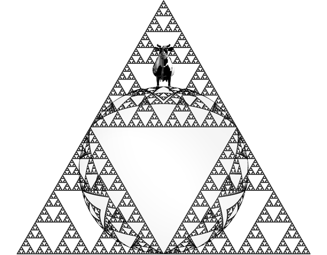
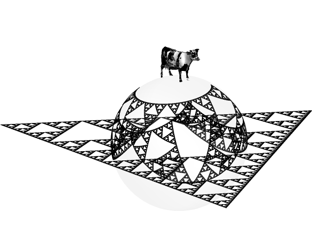
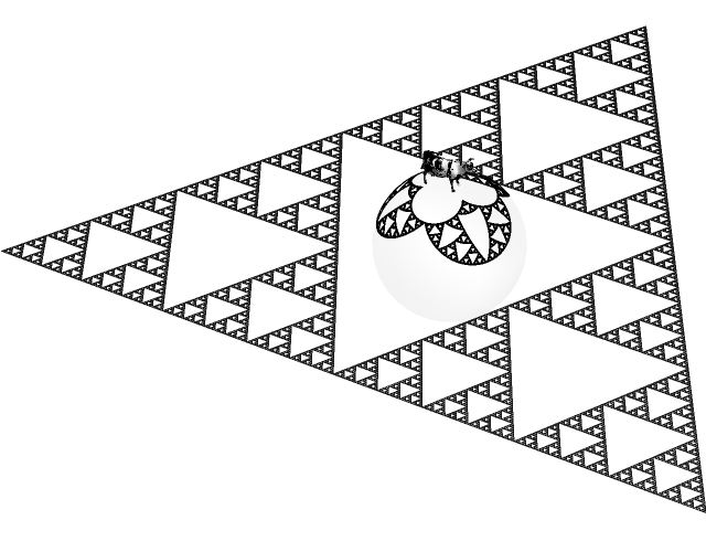
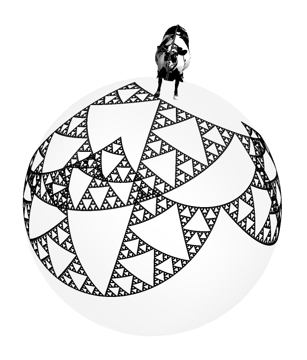
toRiemann = Compile[{{pts, _Real, 2}}, Module[{k},
    Map[(k = 2/(1 + #.#); {k #[[1]], k #[[2]], 1 - k}) &, pts]]];

cow = {EdgeForm[None], Texture[Graphics[Disk[]]], Lighting -> "Neutral",
   Append[ExampleData[{"Geometry3D", "Cow"}, "GraphicsComplex"],
    VertexTextureCoordinates -> 1/500 ExampleData[{"Geometry3D", "Cow"}, "PolygonData"]]};

riemannize[Graphics[g_, ___], options___] := Graphics3D[{
    (*sphere*){Lighting -> "Neutral", Opacity[.07], Sphere[{0, 0, 0}, 1]},
    (*cow*)Rotate[Rotate[Translate[cow, {0, 0, 1.2}], -Pi/2, {0, 0, 1}], -Pi/ 2, {1, 0, 0}],
    (*curves*)g /. (h : Line | Polygon)[pts_] :> {h[{##, 0} & @@@ pts], h[toRiemann[pts]]}},
   options, Boxed -> False];

axiom = Polygon[2 {Cos[#], Sin[#]} & /@ (Pi/2 - 2 Pi Range[3]/3)];

next[prev_] := prev /. Polygon[{p1_, p2_, p3_}] :> {
     Polygon[{p1, (p1 + p2)/2, (p1 + p3)/2}],
     Polygon[{p2, (p2 + p3)/2, (p1 + p2)/2}],
     Polygon[{p3, (p1 + p3)/2, (p2 + p3)/2}]};

draw[n_] := Graphics[{Transparent, EdgeForm[Black], Nest[next, N@axiom, n]}];

riemannize[draw[5], ViewPoint -> Top]