Part 1: https://community.wolfram.com/groups/-/m/t/3531342

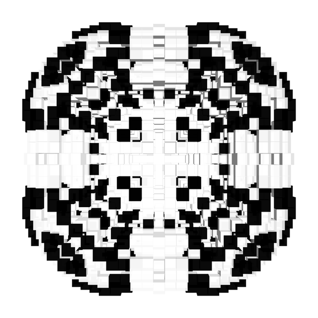
Look at the symmetry of this inversion:

toRiemann = Compile[{{pts, _Real, 2}}, Module[{k},
    Map[(k = 2/(1 + #.#); {k #[[1]], k #[[2]], 1 - k}) &, pts]]];

fromRiemann = Compile[{{pts, _Real, 2}}, Module[{k},
    Map[(-1/(#[[3]] - 1)) {#[[1]], #[[2]], 0} &, pts]]];

cow = {EdgeForm[None], Texture[Graphics[Disk[]]], Lighting -> "Neutral",
   Append[ExampleData[{"Geometry3D", "Cow"}, "GraphicsComplex"],
    VertexTextureCoordinates -> 1/500 ExampleData[{"Geometry3D", "Cow"}, "PolygonData"]]};

riemannTableau[Graphics[g_, ___], options___] := Module[{tmp},
   Graphics3D[{
     Translate[cow, {0, 0, 1.2}],
     {Opacity[.07], Sphere[{0, 0, 0}, 1]},
     g /. (h : Line | Polygon)[pts_] :> {
        EdgeForm[Opacity[.3]],
        (*original*)EdgeForm[Purple], Purple, h[{#1, #2, 0} & @@@ pts],
        (*riemann*)EdgeForm[Blue], Blue, h[tmp = toRiemann[pts]],
        (*riemann inverse*)EdgeForm[Red], Red, h[tmp = {#1, #2, -#3} & @@@ tmp],
        (*inverse*)h[fromRiemann[tmp]]}},
    options, Lighting -> "Neutral", Boxed -> False,
    Axes -> None, PlotRange -> All]];

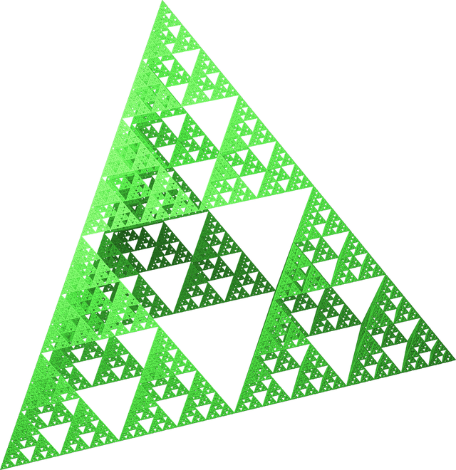
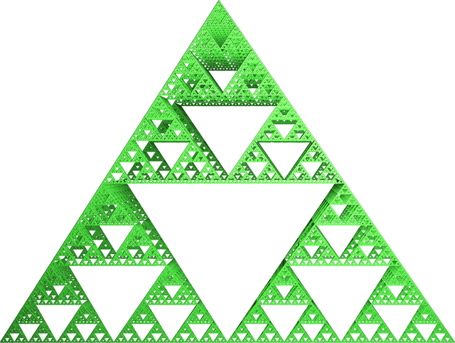
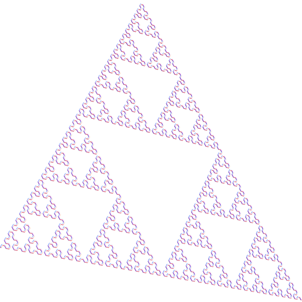
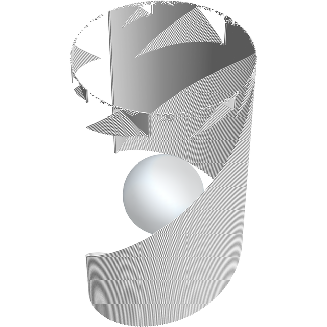
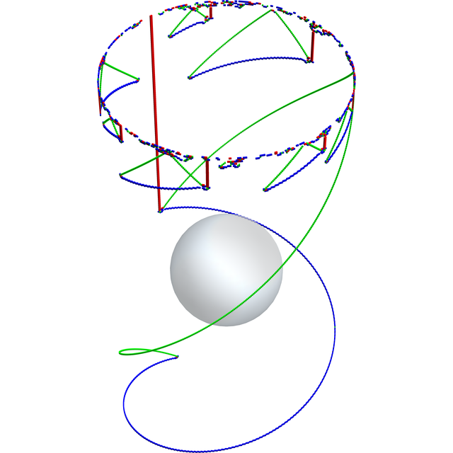
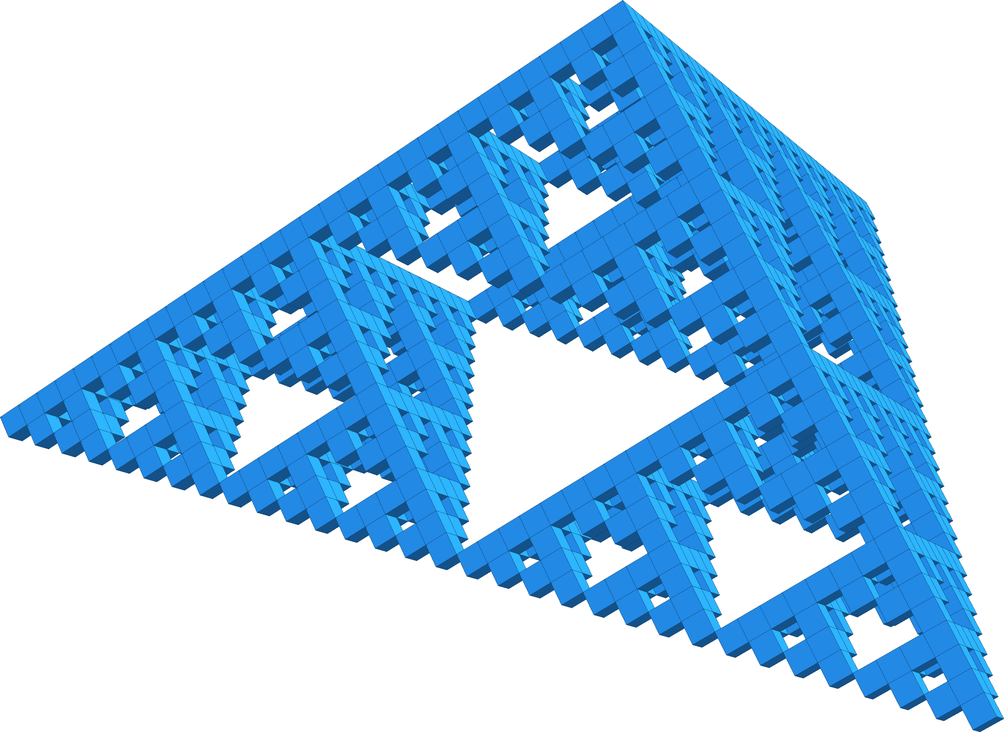
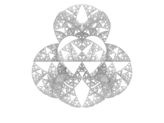
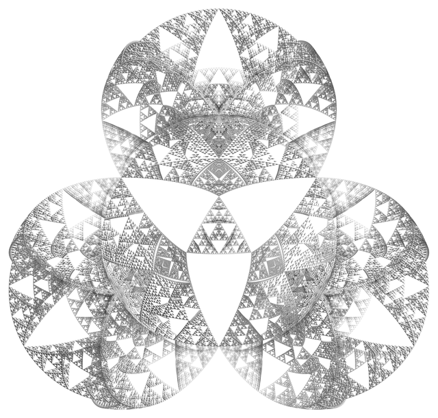
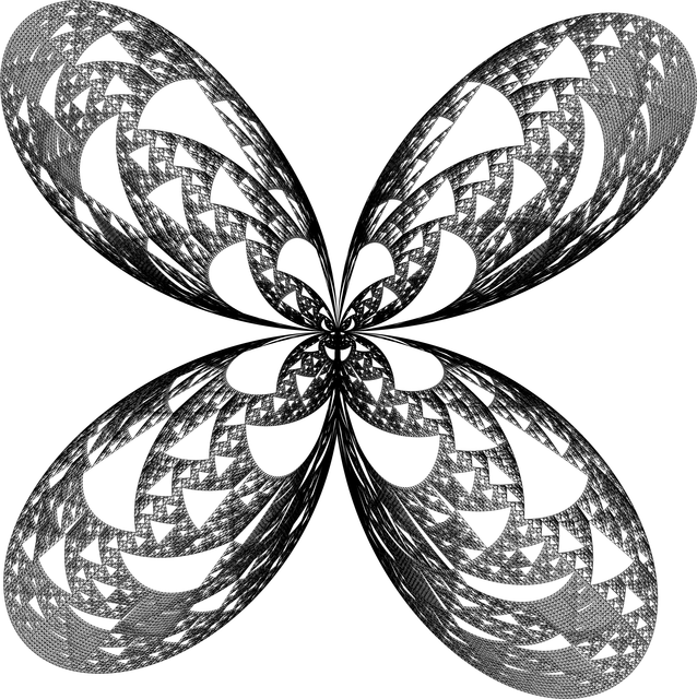
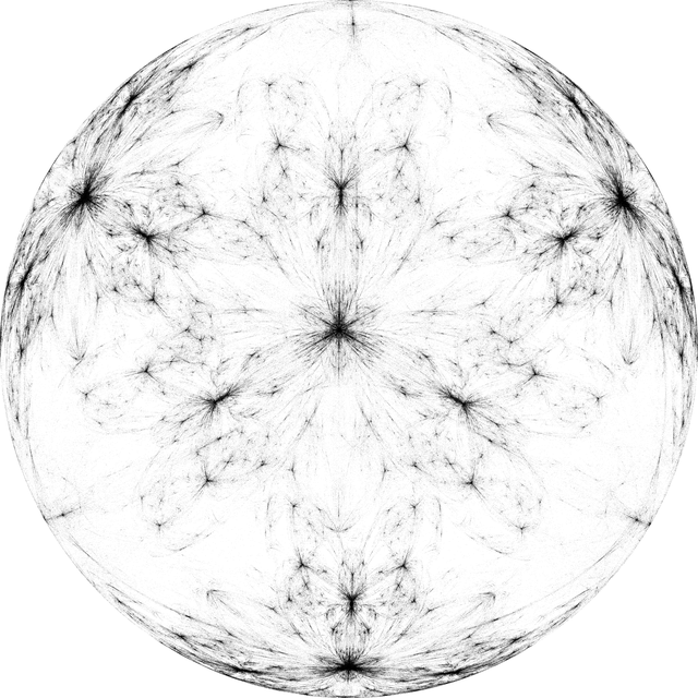
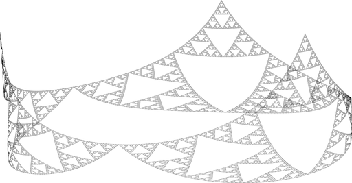
axiom = Polygon[{Cos[#], Sin[#]} & /@ (Pi/2 - 2 Pi Range[3]/3)];

next[prev_] := prev /. Polygon[{p1_, p2_, p3_}] :> {
     Polygon[{p1, (p1 + p2)/2, (p1 + p3)/2}],
     Polygon[{p2, (p2 + p3)/2, (p1 + p2)/2}],
     Polygon[{p3, (p1 + p3)/2, (p2 + p3)/2}]};

draw[n_] := Graphics[Nest[next, N@axiom, n]];

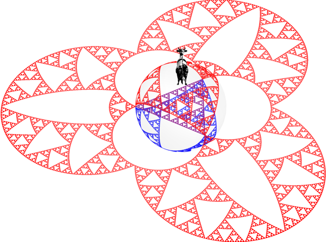
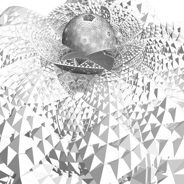
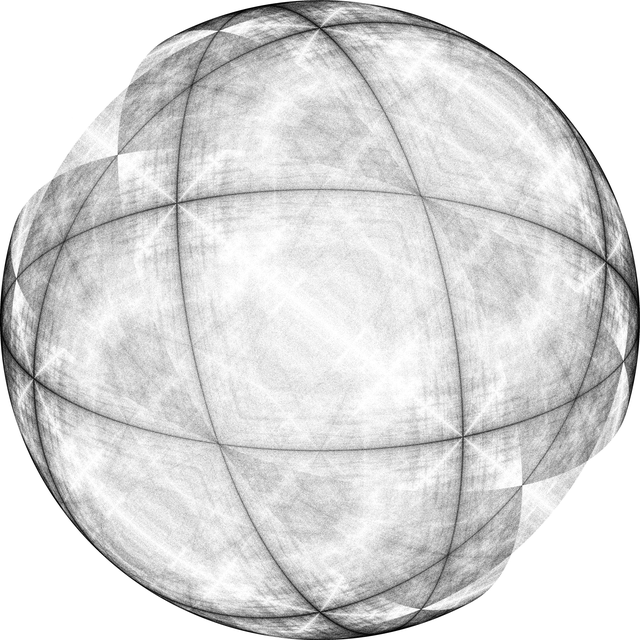
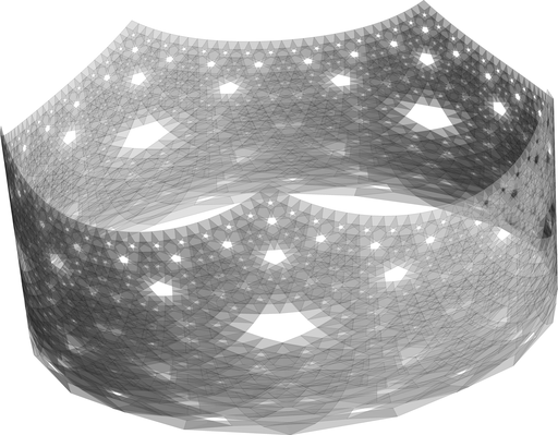
riemannTableau[draw[5], ViewPoint -> {Top, Left}]

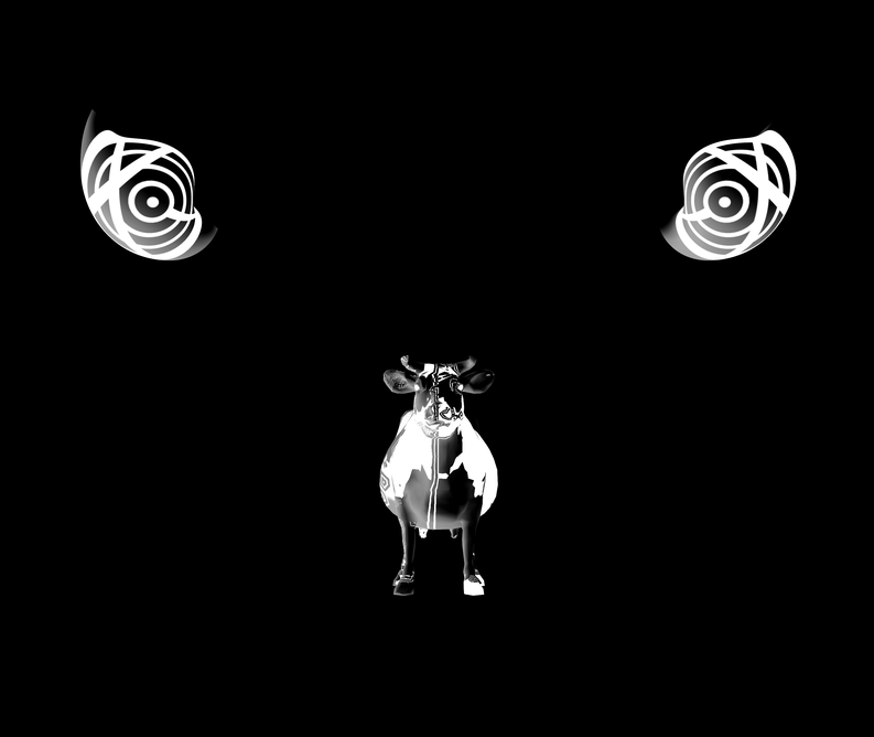
We have the original in the middle in purple, its Riemann mapping in blue, their inverses in red, and the cow in black and white. And except for the cow they all meet at the same three points. How gangster is that. (My friend's six-month old informs me that it's "substantially gangster" (paraphrasing)). But witness the scene of a zoom-out fractal:

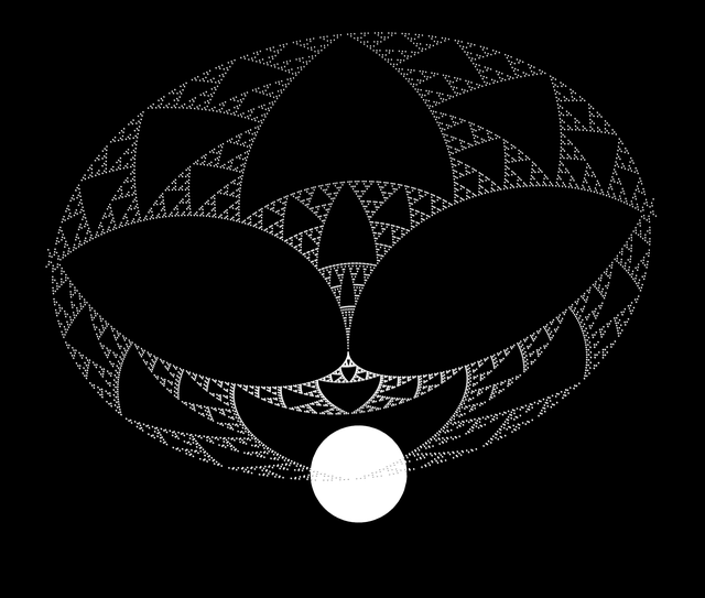
toRiemann = Compile[{{pts, _Real, 2}}, Module[{k},
    Map[(k = 2/(1 + #.#); {k #[[1]], k #[[2]], 1 - k}) &, pts]]];

fromRiemann[pts_] :=
  Quiet@DeleteCases[(-1/(#3 - 1)) {#1, #2, 0} & @@@ pts,
    x_ /; MemberQ[x, Indeterminate]];

cow = {EdgeForm[None], Texture[Graphics[Disk[]]],
   Append[ExampleData[{"Geometry3D", "Cow"}, "GraphicsComplex"],
    VertexTextureCoordinates -> 1/500 ExampleData[{"Geometry3D", "Cow"}, "PolygonData"]]};

riemannTableau[Graphics[g_, ___], options___] := Module[{tmp},
   Graphics3D[{
         (*transparency on sphere causes weird graphical
          issue on my machine when n is high*)
     {Opacity[.07], Sphere[{0, 0, 0}, 1]},
     Translate[cow, {0, 0, 1.2}],
     g /. (h : Line | Polygon)[pts_] :> {
        (*original*)h[{#1, #2, 0} & @@@ pts],
        (*riemann*)h[tmp = toRiemann[pts]],
        (*riemann inverse*)h[tmp = {#1, #2, -#3} & @@@ tmp],
        (*inverted*)h[fromRiemann[tmp]]}},
    options, Lighting -> "Neutral", Boxed -> False,
    Axes -> None, PlotRange -> All]];

next[prev_] := prev /. Polygon[{p1_, p2_, p3_}] :> {
     Polygon[{p1, (p1 + p2)/2, (p1 + p3)/2}],
     Polygon[{p2, (p2 + p3)/2, (p1 + p2)/2}],
     Polygon[{p3, (p1 + p3)/2, (p2 + p3)/2}]};

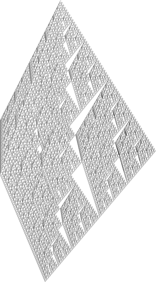
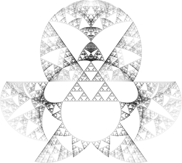
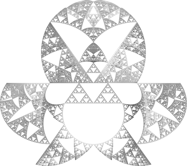
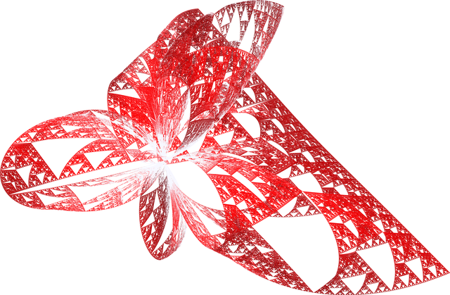
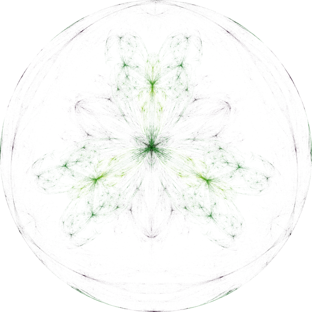
{n, c} = {5, {0, -5/8; -1/4}};
axiom = Polygon[c + {Cos[#], Sin[#]} & /@ (Pi/2 - 2 Pi Range[3]/3)];

riemannTableau[
 Graphics[{EdgeForm[Black], Black, Nest[next, N@axiom, n]}],
 ViewVector -> {5 {-1, -1, 1}, {0, 0, 0}}]

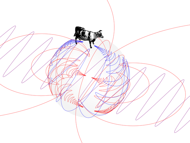
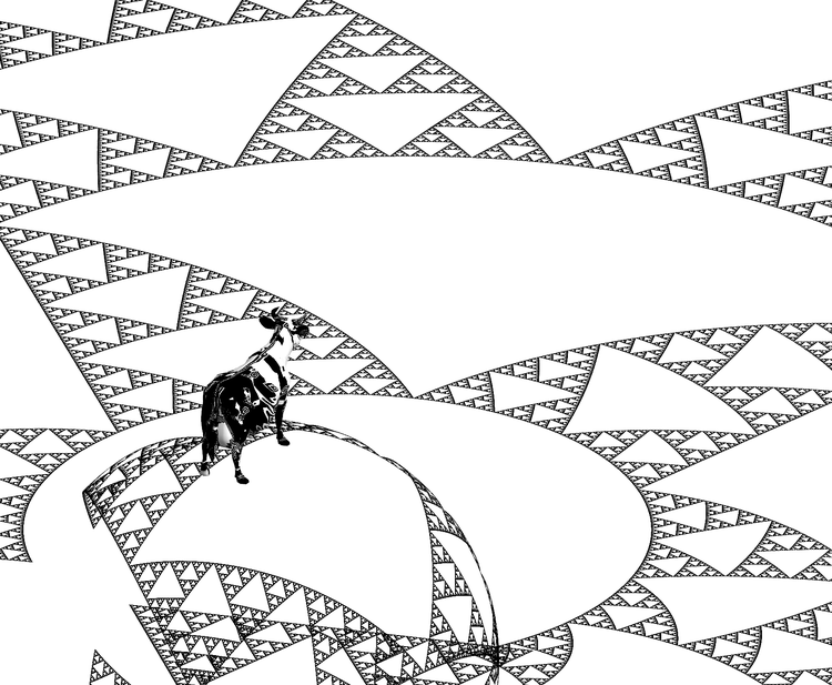
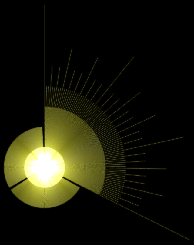
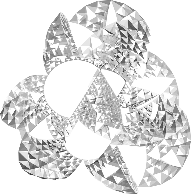
At the chasm of infinity, our cow glances past its precipice, stares down its abyss. You know that machine in the Hitchhiker's Guide that explodes your mind or whatever by showing you how pathetically insignificant you are compared to the universe? Well this is like a Windows 3.1 version of that. Our poor cow friend's soul is being wrung on the very clothesline of endlessness itself. I think this is the first time I'm happy I'm not a cow.

...is what I would have said if this was any cow but this one.

pat = Graphics[{Black, Disk[{0, 0}, 5], White,
    EdgeForm[{Black, Thickness[.03]}],
    Disk[{0, 0}, # + .07] & /@ Range[4, 1, -1],
    Black, Disk[{0, 0}, .15], Rectangle[{-4, 1.8}, {4, 2.1}],
    Rotate[Rectangle[{-4, 1.8}, {4, 2.1}], -Pi/4, {0, 0}],
    Rectangle[{-.2, -1.3}, {.2, -4}]}];

(jhgn = {Lighting -> "Neutral", #1}) & @@
  SphericalPlot3D[u + v, {u, 0, Pi}, {v, 0, Pi},
   Mesh -> None, TextureCoordinateFunction -> ({#5, #4} &),
   PlotStyle -> Texture[pat]];


xf1 = {
   {{0.0017206308062546146`, 0.0012959917814960697`, 0.0025851614902868744`},
    {0.0010674250900446086`, -0.0030803612062593683`, 0.0008337886519470046`},
    {0.0026876120080307113`, 0.0003937069230620502`, -0.0019861927280659755`}},
   {0.3257382788099915`, -0.03759999999999997`, 0.1862691804107692`}};

xf2 = {
   {{0.0017206308062546146`, 0.0012959917814960697`, 0.0025851614902868744`},
    {-0.0010674250900446086`, 0.0030803612062593683`, -0.0008337886519470046`},
    {0.0026876120080307113`, 0.0003937069230620502`, -0.0019861927280659755`}},
   {0.3257382788099915`, 0.03759999999999997`, 0.1862691804107692`}};

cow = {EdgeForm[None], Lighting -> "Neutral",(*Opacity[.999],*) Texture[Graphics[Disk[]]],            
   Append[ExampleData[{"Geometry3D", "Cow"}, "GraphicsComplex"],
    VertexTextureCoordinates -> 1/500 ExampleData[{"Geometry3D", "Cow"}, "PolygonData"]]};

Graphics3D[{cow,
  GeometricTransformation[jhgn, xf1],
  GeometricTransformation[jhgn, xf2]},
 Boxed -> False]

pat =(*ColorNegate@*)Graphics[{Black, Disk[{0, 0}, 5], White,
    EdgeForm[{Black, Thickness[.03]}],
    Disk[{0, 0}, # + .07] & /@ Range[4, 1, -1],
    Black, Disk[{0, 0}, .15], Rectangle[{-4, 1.8}, {4, 2.1}],
    Rotate[Rectangle[{-4, 1.8}, {4, 2.1}], -Pi/4, {0, 0}],
    Rectangle[{-.2, -1.3}, {.2, -4}]}];

(jhgn = {Lighting -> "Neutral", #1}) & @@
  SphericalPlot3D[u + v, {u, 0, Pi}, {v, 0, Pi},
   Mesh -> None, TextureCoordinateFunction -> ({#5, #4} &),
   PlotStyle -> Texture[pat], PlotPoints -> 80(*0*)];

sc = 1.5;
xf1 = {
   sc {{0.010433915075096155`, 0.02050184708176941`, -0.0014526467022039392`},
     {0.014609900826184952`, -0.006252356712311273`, 0.01669614726190017`},
     {0.014456372783472383`, -0.008478490536514085`, -0.01582501134810082`}},
   {0.5447560973768777`, -0.5`, 0.5534681561478464`}};

xf2 = {
   sc {{0.010433915075096155`, 0.02050184708176941`, -0.0014526467022039392`},
     {-0.014609900826184952`, 0.006252356712311273`, -0.01669614726190017`},
     {0.014456372783472383`, -0.008478490536514085`, -0.01582501134810082`}},
   {0.5447560973768777`, 0.5`, 0.5534681561478464`}};

cow = {EdgeForm[None], Lighting -> "Neutral",(*Opacity[.999],*) Texture[ColorNegate@Graphics[Disk[]]],
   Append[ExampleData[{"Geometry3D", "Cow"}, "GraphicsComplex"],
    VertexTextureCoordinates -> 1/500 ExampleData[{"Geometry3D", "Cow"}, "PolygonData"]]};

Graphics3D[{cow,
  GeometricTransformation[jhgn, xf1],
  GeometricTransformation[jhgn, xf2]},
 ViewPoint -> Right, Boxed -> False] // ColorNegate

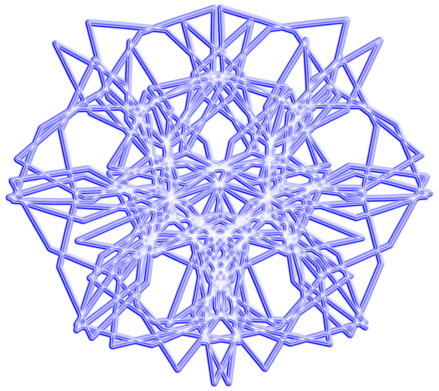
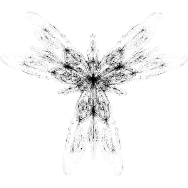
This cow does not cower. Infinity cannot bully this bull, cannot bloviate this bovine. By all appearances this cow is wearing infinity on its mane. Its horns are probably made of ℵℵ⋱ down 4 or 5 levels, an immutability surpassed only by that of the tusks of the Alephant. Our cow isn't staring into infinity. It's looking down at infinity, observing infinity with detached understanding. If our cow were not so enlightened, and also had the facial muscles, it might betray the subtlest of smiles at infinity's infinity face, for infinity's turbid fractal whirlpools and vast lethargic swamps are but swathes of data like any other to this cow.

Long ago, having mastered the magesterial tetrafecta of science, mathematics, spirituality, and politics, our cow stepped hoof outside Farmer Joe's farm and set out on an adventure of like, just so much awesome. One of its side gigs these days is being the final observer of our domain, preventing our section of the Great Algorithm from backtracking by stellating through the cosmos our most entwined entwinements. I think this is the first time I'm jealous of a cow.

In any case, as you can see the Riemann sphere is pretty useless. But while we're on the subject of 3D let's see how our various approaches do here. Chaos game:

draw[vertices_, numPoints_, options___] :=
  Graphics3D[{Lighter[Green],
    Sphere[FoldList[(#1 + #2)/2 &, First[N@vertices],
      RandomChoice[N@vertices, numPoints]], .001]},
   Lighting -> {{"Point", LightYellow, Scaled[{1, 1, 1}], 5}},
   options, Boxed -> False];

vertices = PolyhedronData[{"Pyramid", 3}, "VertexCoordinates"];
draw[vertices, 100000,
 ViewPoint -> {0, 0, Infinity},
 ViewVertical -> {1, 0, 0}]

draw1[vertices_, numPoints_, options___] :=
  Graphics3D[{Lighter[Green], EdgeForm[None],
    Cuboid[#, # + .01] & /@ FoldList[(#1 + #2)/2 &, First[vertices],
      RandomChoice[N@vertices, numPoints]]},
   Lighting -> {{"Point", LightYellow, Scaled[{1, 1, 1}], 5}},
   options, Boxed -> False];

draw[vertices_, numPoints_, options___] :=
  Graphics3D[{Lighter[Green],
    Sphere[FoldList[(#1 + #2)/2 &, First[N@vertices],
      RandomChoice[N@vertices, numPoints]], .001]},
   Lighting -> {{"Point", LightYellow, Scaled[{1, 1, 1}], 5}},
   options, Boxed -> False];

vertices = PolyhedronData[{"Pyramid", 3}, "VertexCoordinates"];

(*1*)
Defer[AbsoluteOptions][draw1[vertices, 20000, ImageSize -> Medium]]

(*2*)
draw[vertices, 2000000,
   (* ViewPoint, ViewVertical from (*1*) *)
   Method -> {"ShrinkWrap" -> True},
   ImageSize -> 2 1280] // Rasterize // ImageResize[#, Scaled[1/4]] &

This is using little spheres as the points. You could use pyramids or anything else instead. Even go back to nature and use actual points. It's a bit tricky to get decent images since the chaos game doesn't place points in a regular arrangement, so you need a large number of points. Each of these images uses 2 million spheres and takes about 10 minutes to render on my little laptop.

This top view shows one of the symmetries that appear in the 3D triangle. This side view shows another. And a top view of the 4-corner pyramid. These symmetries are interesting because they appear absolutely no different than 2D renditions (for example). At first this seems mysterious, since the symmetries appear from every which angle. But the reason it happens is because our distance function works on each coordinate independently:

$$p_{i+1}=\frac{1}{2} (p_i+\nu)$$

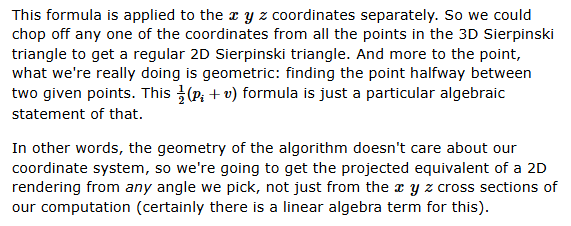
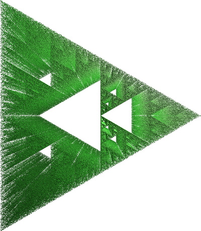
To make clear what we're talking about, this is the chaos game on a prism, and the same thing from the same viewpoint, except with the 3D projection effect removed. As you can see, the 'hidden dimension' has no offect on what is seen. Au contraire messieur. If it did have an effect, that would be interesting.

Something I noticed though is that while we can remove a coordinate, we can't add a coordinate, in the sense that, for example, there's no way to combine independent $x$ $y$ streams to create a Sierpinski triangle. For our 2D Sierpinski triangle, there's something to the fact that a single point is specified by two coordinates instead of just one.

I think there may be an interesting statistical or information-theoretic interpretation to this. I'm not really familiar with either of these subjects though. Geometric approach:

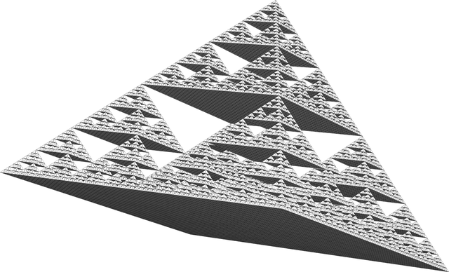
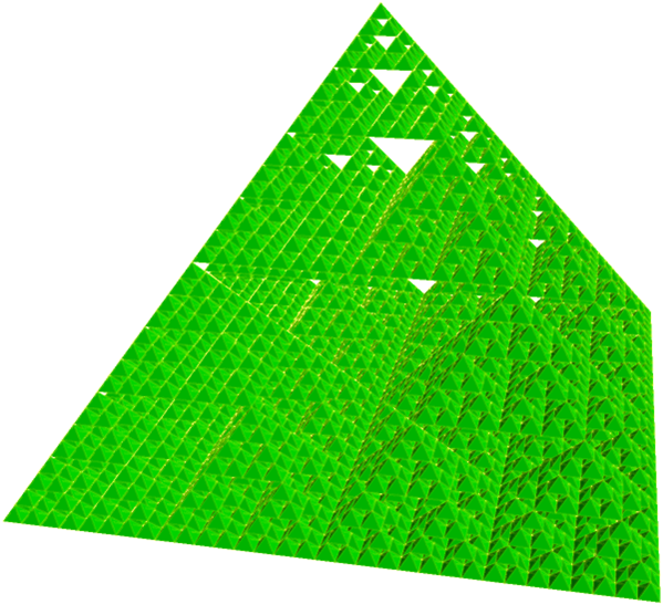
draw[shapeName_, n_, options___] := Module[{shape, next},
   shape = PolyhedronData[shapeName, "Faces"];

   (*scale by 1/2 toward each vertex,in turn*)
   next[prev_] := Scale[prev, 1/2, #] & /@ shape[[1]];

   Graphics3D[{EdgeForm[Opacity[.15]], Nest[next, N@shape, n]},
    options, Lighting -> "Neutral", Boxed -> False]];

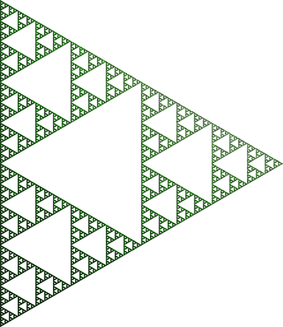
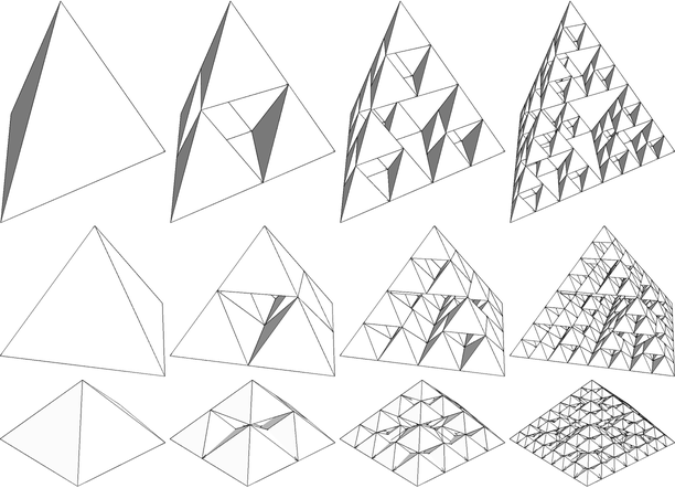
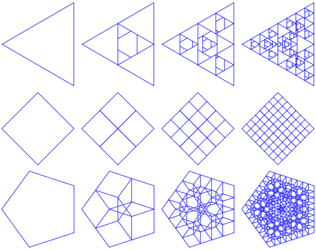
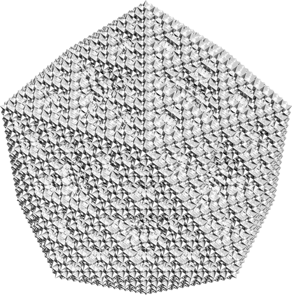
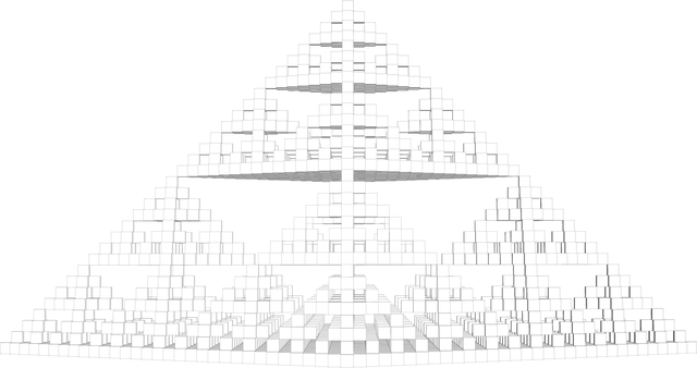
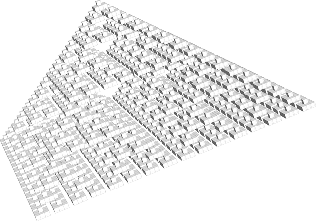
Grid[Table[
  draw[{"Pyramid", k}, n, ViewPoint -> {0, 0, Infinity}],
  {k, 3, 5}, {n, 0, 3}]]

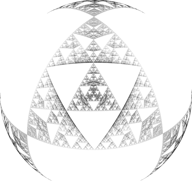
Behold the Lemon Lime Fortress. Throw in a few salt blocks, pour some Corona at the top, join the party at the base. To make our lives one notch easier, our code takes advantage of Mathematica's built-in transformation infrastructure, in this case the symbol Scale. It also pulls the geometry of things from our good friend Mr. PolyhedronData. The nice thing about having such a general setup is that we can readily apply this geometric fractalization on arbitrary shapes:

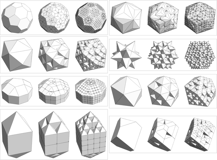
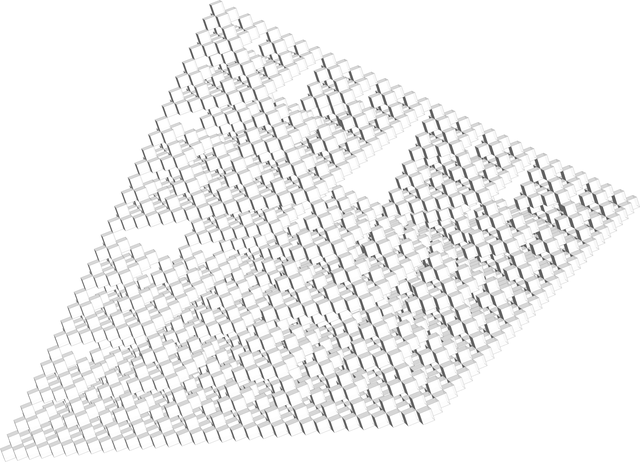
draw[shapeName_, n_] := Module[{shape, next},
   shape = PolyhedronData[shapeName, "Faces"];
   next[prev_] := Scale[prev, 1/2, #] & /@ shape[[1]];

   Graphics3D[Nest[next, N@shape, n],
    Method -> {"ShrinkWrap" -> True},
    Lighting -> "Neutral", Boxed -> False]];

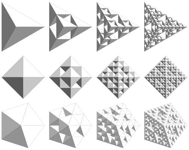
shapes = {"TruncatedIcosahedron", "TriakisIcosahedron", "TetrakisHexahedron",
   "SmallStellatedDodecahedron", "ElongatedPentagonalCupola", "Icosahedron",
   "ElongatedSquareDipyramid", "DuerersSolid"};

Grid[Partition[#, 2]] &[
 Table[Tooltip[Panel[#], shape] &@
   Row[Table[draw[shape, n], {n, 0, 1}], Spacer[30]],
  {shape, shapes}]]

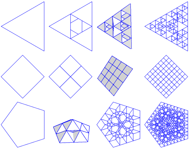
Don't ask me what the hell that last shape is. I figure it just managed to stow away into PolyhedronData somehow, like the semiconscious pre-sentient kernel of a future Skynet. The faces of these shapes show very clearly that we get 2D slices for free, like in these perspectives from below (we aren't cheating here). The edges by themselves make pretty patterns:

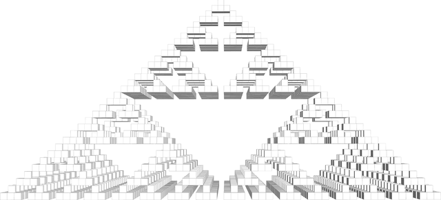
draw[shapeName_, n_, options___] := Module[{shape, next, axiom},
   shape = PolyhedronData[shapeName, "Faces"];
   next[prev_] := Scale[prev, 1/2, #] & /@ shape[[1]];

   axiom = {shape, If[showLittleBalls,
      {FaceForm[{Opacity[.85], White}],
       Glow[Green], Sphere[{0, 0, 0}, .09]}]};

   Graphics3D[{Transparent, EdgeForm[{Opacity[opacity], color}],
     Nest[next, N@axiom, n]}, options, Lighting -> "Neutral",
    Boxed -> False]];

shapes = {"TruncatedIcosahedron", "TriakisIcosahedron", "TetrakisHexahedron",
   "SmallStellatedDodecahedron", "ElongatedPentagonalCupola", "Icosahedron",
   "ElongatedSquareDipyramid", "DuerersSolid"};

{color, opacity, showLittleBalls} = {Black, .6, False};
Grid[Partition[#, 2]] &@
 Table[Tooltip[#, shape] &@
   Row[Table[draw[shape, n, ViewPoint -> Top], {n, 0, 1}], Spacer[30]],
  {shape, shapes}]

To make sure that after all this scrolling we're still on the same web page, this is our chaos game algorithm:

1 start at any point. call it p
2 pick a vertex at random
3 find the point halfway between p and that vertex
4 call that point p and draw it
5 goto 2

The only difference between 2D and 3D versions of this algorithm is having 3 coordinates instead of 2. Just as in 2D, we can alter step 3 in various ways. The simplest is to move not halfway towards the chosen vertex, but .25 or .7 of the way, etc:

draw[vertices_, df_, numPoints_, options___] := Graphics3D[{
    Opacity[.5], PointSize[0],
    Point[FoldList[df, First[N@vertices],
      RandomChoice[N@vertices, numPoints]]]},
   (*Method->{"ShrinkWrap"->True},*)
   options, PlotRange -> Automatic, Boxed -> False];

functions = Function[r, r (#1 + #2) &] /@ {1, .96, .6, .5, .2};

Grid[Join[
  {TraditionalForm[Trace[#[a, b]][[2]]] & /@ functions},
  ParallelTable[
   draw[PolyhedronData[{"Pyramid", v}, "VertexCoordinates"],
    df, 50000, ViewPoint -> {Front, Top}],
   {v, 3, 5}, {df, functions}]]]

Those odd random walks are because the 4- and 5-pyramids have Mean[vertices] != {0, 0, 0}. One thing I noticed is that random walks resemble the outlines of continents. How curious. I wonder if it boils down to the self-similarity of the Brownian motion of water molecules, or something of the like. I.e. the idea that if our continents were surrounded by materials which did not move Brownianly, our coastlines would have different kinds of shapes. Remember that we can get creative with our distance function:

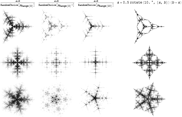
draw[vertices_, df_, numPoints_, options___] :=
  Graphics3D[{PointSize[0], Opacity[.3],
    Point[FoldList[df, RandomReal[{0, .0001}, 3],
      RandomChoice[N@vertices, numPoints]]]},
   (*Method->{"ShrinkWrap"->True},*)
   options, Boxed -> False];

rotate = RotationTransform;
functions = {
   (#1 + #2)/RandomChoice[Prime[Range[3]]] &,
   (#1 + #2)/RandomChoice[Prime[Range[3]]!] &,
   (#1 + #2)/RandomChoice[Prime[Range[10]]] &,
   #1 + .5 rotate[10. Degree, {#1, #2}][#2 - #1] &};

Grid[Join[
  {TraditionalForm[Trace[#[a, b]][[2]]] & /@ functions},
  ParallelTable[
   draw[PolyhedronData[{"Pyramid", v}, "VertexCoordinates"], df, 5000],
   {v, 3, 5}, {df, functions}]]]

game = Compile[{{vertices, _Real, 2}, {w, _Real}, {numpoints, _Integer}},
   Module[{diff},
    FoldList[(diff = #2 - #1;
       Clip[(#1 + #2) Log[Sqrt[diff.diff] + w]]) &,
     {0, 0, 0}, RandomChoice[vertices, numpoints]]]];

draw[vertices_, w_, numPoints_, options___] :=
  Graphics3D[{PointSize[0], Opacity[7 .05],
    Point[game[vertices, w, numPoints]]},
   options, Boxed -> False];

Needs["PolyhedronOperations`"];
vertices = Stellate[PolyhedronData[{"Pyramid", 5}, "Faces"]][[1]];

draw[vertices, .2, 600000, PlotRange -> All(*,
 Method->{"ShrinkWrap"->True}*)(*,ViewPoint->{Infinity,0,0}*)]

These pictures differ by w factor, viewpoint, or the set of vertices on which the game is being played. For most of these I'm using the vertices of regular polyhedra from PolyhedronData. Note that the vertices of the game are not necessarily in proportion to the figure itself.

At this point I should remention that all of the code snippets on this page are self-contained. If you have Mathematica you can copy-paste this and start producing these figures, which, I should also remention, are interactive 3D models. I'm a big fan of black ink on white paper, and these are like being able to change the perspective of a pure ink painting in real time. Teknikara no jutsu.

game = Compile[{{vertices, _Real, 2}, {w, _Real}, {numpoints, _Integer}},
   Module[{diff},
    FoldList[(diff = #2 - #1;
       Clip[(#1 + #2) Log[Sqrt[diff.diff] + w]]) &,
     {0, 0, 0}, RandomChoice[vertices, numpoints]]]];

draw[vertices_, w_, numPoints_, options___] :=
  Graphics3D[{PointSize[0], Opacity[7 .05],
    Point[game[vertices, w, numPoints]]},
   options, Boxed -> False];

proc[img1_, cf_: ColorData[1], mode_: None, blur_: 8] :=
  Module[{img, components, rank, largest, colored},
   img = RemoveAlphaChannel[ColorNegate@ColorConvert[img1, "Grayscale"]];
   components = MorphologicalComponents[img];

   Module[{measurements, sorted},
    measurements = ComponentMeasurements[components, "Count"];
    sorted = First /@ Reverse@SortBy[measurements, Last];
    rank[label_] := (rank[label] = Position[sorted, label][[1, 1]])];

   colored = Colorize[components,
     ColorFunction -> (cf[rank[#]] &), ColorFunctionScaling -> False];

   If[mode == "Angelic",
    colored = ImageMultiply[img, colored]];

   ColorNegate[ImageMultiply[ColorNegate[img],
       Blur[#, blur] &@ColorNegate[colored]]] // ImageAdjust];

Needs["PolyhedronOperations`"];
vertices = OpenTruncate[PolyhedronData[{"Pyramid", 3}, "Faces"]][[1]];
g = draw[vertices, .5, 600000, Method -> {"ShrinkWrap" -> True}];

proc[g, # /. Join[
    Thread[Range[4] -> {Red, Green, Green, Green}],
    {_ -> Lighter[Green]}] &]

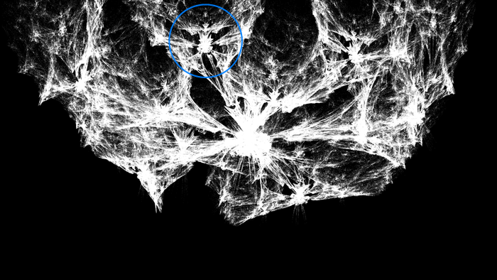
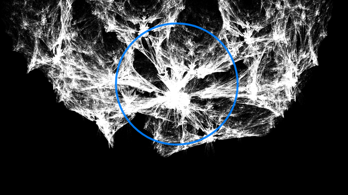
Some of thes are like alien Rorschach tests. Like what do you see in this one? I see a mosquito that can suck the lifeblood out of your soul. This one, however, is definitely from an as-yet unreleased Matrix film. And we also have the Minotaur's armor and his shield of Cancer. I'd recognize my buddy's armor in even the most obtuse alien Rorschachs. See also a stereographic projection of one of the rooms of Asterion's maze and an aspect, which needs no explanation.

The originals are 3D but this coloring is a 2D image process. It highlights components of the image based on their sizes. So if your image has 3 large blobs with dozens of tiny blobs all around, you can use, for example, # /. {1 -> Red, 2 -> Green, 3 -> Yellow, _ -> Pink} & to color the big blobs specific colors and all other blobs pink. Though in most of these images I only use one or two colors.

game = Compile[{{vertices, _Real, 2}, {numPoints, _Integer}, {wowzerz, _Real}},
   Module[{diff},
    FoldList[(diff = #2 - #1;
       Clip[(#1 + #2) Log[Sqrt[diff.diff] + wowzerz]]) &,
     {0., 0., 0.}, RandomChoice[vertices, numPoints]]]];

{numFrames, imageSize, numPoints} = {
    {5(*sec*)15(*fps*), 1/2 {640, 480}, 1/3 600000},
    {20(*sec*)15(*fps*), {640, 480}, 600000}}[[1]];

Needs["PolyhedronOperations`"];
vertices = Stellate[PolyhedronData[{"Pyramid", 5}, "Faces"]][[1]];

frame = Function[w,
   Graphics3D[{Opacity[.1], PointSize[0], Point[game[vertices, numPoints, w]]},
    ImageSize -> imageSize, ViewVertical -> {0, 0, 1}, Boxed -> False, SphericalRegion -> True, PlotRange -> 1,
    ViewVector -> {RotationTransform[2 Pi w, {0, 0, 1}][{1, 0, (w - .25) Pi/2}], {0, 0, 0}}]];

SetDirectory["c:/users/zrp/desktop/frames"];

range = Range[0, 3/4, 3/4/(numFrames - 1)];
file[w_] := ToString[N@w] <> ".png";

ParallelDo[
  If[! FileExistsQ[file[w]],
   Export[file[w], frame[w]]],
  {w, range}];

Export["mov.avi",
 ColorNegate /@ ImageAdjust /@ Import /@ file /@ range]

Beep[];
Button[open, SystemOpen["mov.avi"],
 Enabled -> FileExistsQ["mov.avi"]]

MovieMaker[frameF_, range : {start_Integer, stop_Integer}, rest___] :=
  MovieMaker[frameF, {start, stop, stop - start}, rest];

(*arithmetic for eg doubling movie length is easier by 'intervals' than by 'frame count'*)
MovieMaker[frameF_, range : {start_, stop_, numIntervals_}, rest___] :=
  MovieMaker[frameF, List[Range[#1, #2, (#2 - #1)/#3(*(#3-1)*)] & @@ range], rest];

MovieMaker::expqq = "Export is complaining about something. " <>
   "Most likely you're feeding it items with different image sizes.";

MovieMaker::usage =
  "NOTE: copies of this notebook are automatically stored along
  with the generated files. To prevent this, set AutoArchive -> False.

  MovieMaker[frameFunction, rangeSpec, options___]

  rangeSpec:
  {start, stop, number of intervals}:  {0, 1, 5(*sec*)15(*fps*)}
  {start, stop} integer range:  {1, 20}
  {explicit list}:  {AstronomicalData[\"Earth\",\"OrbitPath\"][[1]]}

  The Label option determines the folder name under which the animation
  is created. For example, if changing a variable X makes a different
  animation, then place that variable in the Label spec so that when you
  change that variable, the animation will be generated in a different folder.

  Likewise, the first element of the Process spec determines the folder
  and uniqueness of the process function. Processes work in subfolders of
  the main project folder, meaning you can experiment with multiple processes
  in a single project.

  MovieMaker[
   {ToLowerCase[#], ToUpperCase[#]} &, {CharacterRange[\" \", \"~\"]},
   Serialization -> Hash, Label -> \"UpperLower\", FileTypes -> {\".mx\", \".png\", \".gif\"},
   Process -> {\"times\", ImageMultiply @@ Map[Rasterize[#, ImageSize -> 400 {1, 1}] &, #] &},
   MovieOptions -> {\"DisplayDurations\" -> 1}, MapFunction -> Map]

  Serialization is for converting values to valid file names.
  MapFunction is for when you don't want to use parallelization.
  Directory setting specifies the specific project folder, overriding Label.";

Options[MovieMaker] = {
   Label -> Automatic, Process -> {None, None}, MapFunction -> ParallelMap, AutoArchive -> True,
   FileTypes -> {".png", ".png", ".avi"}, MakeMovie -> True, MovieOptions -> {}, Directory -> Automatic,
   Ordering -> (BlockRandom[RandomSample[#]] &), Serialization -> Composition[List, Chop, N]};
(* After I wrote this program, a more powerful approach occurred to me. We could have a
macro that would be used something like this: *)
FileBackedProcess[Function[val,
   a = S[1][Rasterize@dirp[val]];
   b = S[2][Rasterize@derp[val]];
   S[3][ImageMultiply[a, b]]]];
(* where the S[i_][body_] are the momoization points into the file system. If the S finds
the file corresponding to the [i][body], then the file is imported. Otherwise it executes
the body and saves the file. The point would be to make the file aspect as
easy as annotating things with S[i] *)

MovieMaker[frameF_, List[valueList_List], OptionsPattern[]] := Module[{
   tooltip, mainLabel, processLabel, processF, mapF, frameExt, processedExt, movieExt, dir,
   framesDir, processedDir, movieFile, fileMap, numFrames, alive = True, folder0exists,
   foldersExistL, folder1exists, folder2exists, progress1, progress2, movieDone, makeFrames,
   processFrames, makeMovie, serialization, archive, makeMovieA, preview, printPreview, printFileMap},

  tooltip[expr_] := Tooltip[#, expr, TooltipDelay -> .25] &;
  {mainLabel, mapF, makeMovieA, serialization} =
   OptionValue[{Label, MapFunction, MakeMovie, Serialization}];

  {processLabel, processF} =
   Replace[OptionValue[Process], {
     {pf_} :> {ToString[pf], pf},
     pf : Except[_List] :> {ToString[pf], pf}}];

  {frameExt, processedExt, movieExt} = PadRight[
    Flatten[List[OptionValue[FileTypes]]], 3,
    FileTypes /. Options[MovieMaker]];

  mainLabel = Replace[mainLabel,
    Automatic -> IntegerString[Hash[{frameF, valueList}, "CRC32"], 36]];
  dir = Replace[OptionValue[Directory], Automatic ->
     FileNameJoin[{NotebookDirectory[], "vids", ToString[mainLabel]}]];

  framesDir = FileNameJoin[{dir, "frames"}];
  processedDir = FileNameJoin[{dir, "processed", ToString[processLabel]}];
  movieFile = FileNameJoin[{dir, ToString[{processLabel, mainLabel}] <> movieExt}];

  (* main iteration construct *)
  fileMap[f_, vals_: valueList, map_: mapF] := map[Function[val,
     f[
      FileNameJoin[{framesDir,
        ToString[serialization[val]] <> frameExt}],
      FileNameJoin[{processedDir,
        ToString[serialization[val]] <> processedExt}],
      val]],
    vals];

  numFrames = Length[valueList];
  progress1 = Total@Boole[fileMap[FileExistsQ[#1] &]];
  progress2 = Total@Boole[fileMap[FileExistsQ[#2] &]];
  foldersExistL = FileExistsQ /@ {dir, framesDir, processedDir};
  movieDone = FileExistsQ[movieFile];
  SetSharedVariable[progress1, progress2];

  If[OptionValue[AutoArchive] && FileExistsQ[dir] &&
    ! FileExistsQ[FileNameJoin[{dir, ToString[mainLabel] <> ".nb"}]],
   Export[FileNameJoin[{dir, ToString[mainLabel] <> ".nb"}],
    NotebookGet[EvaluationNotebook[]]]];
(**)
makeFrames[] := (
   Quiet@CreateDirectory[framesDir];
   foldersExistL[[1 ;; 2]] = {True, True};
   If[OptionValue[AutoArchive],
    Export[FileNameJoin[{dir, ToString[mainLabel] <> ".nb"}],
     NotebookGet[EvaluationNotebook[]]]];

   fileMap[If[! FileExistsQ[#1],
      Export[#1, frameF[#3]];
      progress1++] &,
    OptionValue[Ordering][valueList]]);

(**)
processFrames[] := If[
   processF =!= None,
   Quiet@CreateDirectory[processedDir];
   foldersExistL[[3]] = True;
   If[OptionValue[AutoArchive],
    Export[FileNameJoin[{processedDir, ToString[{mainLabel, processLabel}] <> ".nb"}],
     NotebookGet[EvaluationNotebook[]]]];

   fileMap[If[! FileExistsQ[#2] && FileExistsQ[#1],
      Export[#2, processF[Import[#1]]];
      progress2++] &,
    OptionValue[Ordering][valueList]]];

(**)
makeMovie[] := If[makeMovieA,
   If[FileExistsQ[movieFile],
    Print["movie file already exists"],
    With[{ab = If[processF === None, #1, #2]},
     If[And @@ fileMap[FileExistsQ[ab] &],
      Check[
        Export[movieFile, fileMap[Import[ab] &],
         Sequence @@ OptionValue[MovieOptions]];
        movieDone = True, Message[MovieMaker::expqq];
        movieDone = False, {Export::errelem}]]]]];

(**)
preview[] := preview[RandomChoice[valueList]];
preview[val_] := Module[{frame, fileName, tempFile},
   tempFile = FileNameJoin[{$TemporaryDirectory, ToString[Hash[val]] <> frameExt}];
   fileName = First@fileMap[#1 &, {val}];

   If[FileExistsQ[fileName],
    (**)frame = Import[fileName],
    (**)frame = Import[Export[tempFile, frameF[val]]];
    Print[Labeled[frame, N@val, Right]]; Beep[]];

   If[processF =!= None,
    Print[Labeled[processF[frame], N@val, Right]]; Beep[]]];

(**)
printPreview[] := CellPrint[ExpressionCell[Defer[
     preview[Placeholder["val"]]], "Input"]];

(**)
printFileMap[] := CellPrint[ExpressionCell[Defer[
     frames2 = fileMap[If[FileExistsQ[#2], Import[#2], Sequence @@ {}] &];],
    "Input"]];

(**)
archive[] := Module[{fileName},
   fileName = ToString[mainLabel] <> " " <>
     DateString[{"DateShort",
       " (", "Hour12", " ", "Minute", " ", "Second", " ", "AMPM", ")"}];

   Quiet@CreateDirectory[dir];
   foldersExistL[[1]] = True;
   Export[FileNameJoin[{dir, fileName <> ".nb"}],
    NotebookGet[EvaluationNotebook[]]];

   Beep[]];
(*controls*)
  With[{
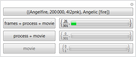
    btnMakeFrames = Button["frames + process + movie",
      makeFrames[]; Beep[]; processFrames[]; Beep[]; makeMovie[]; Beep[],
      Method -> "Queued", Enabled -> Dynamic[progress1 =!= numFrames]],
    btnProcessFrames = Button["process + movie",
      processFrames[]; Beep[]; makeMovie[]; Beep[],
      Method -> "Queued", Enabled -> Dynamic[
        progress2 =!= numFrames && progress1 =!= 0 && processF =!= None]],
    btnMakeMovie = Button["movie",
      makeMovie[]; Beep[],
      Method -> "Queued", Enabled -> Dynamic[
        (progress2 === numFrames ||
           (processF === None && progress1 === numFrames)) &&
         ! movieDone && makeMovieA]],
    btnMainFolder = tooltip["open folder"]@
      Button[{mainLabel, processLabel}, SystemOpen[dir],
       Enabled -> Dynamic[foldersExistL[[1]]]],
    btnFramesFolder = tooltip["open folder"]@
      Button[{Dynamic[progress1]/ToString[numFrames],
        ProgressIndicator[Dynamic[progress1/numFrames]]},
       SystemOpen[framesDir],
       Enabled -> Dynamic[foldersExistL[[2]]]],
    btnProcessFolder = tooltip["open folder"]@
      Button[{Dynamic[progress2]/ToString[numFrames],
        ProgressIndicator[Dynamic[progress2/numFrames]]},
       SystemOpen[processedDir],
       Enabled -> Dynamic[processF =!= None && foldersExistL[[3]]]],
    btnMovieFile = tooltip["open movie"]@
      Button[{Dynamic[Boole[movieDone]]/"1",
        ProgressIndicator[Dynamic[Boole[movieDone]/1]]},
       SystemOpen[movieFile], Enabled -> Dynamic[movieDone]]},

   (*without going the extra mile, better to have no persistence*)
   Dynamic[If[alive === True,
       Panel[#, FrameMargins -> {{Automatic, Automatic}, {Automatic, 0}}],
       Panel[Tooltip[Overlay[{
           Style["VWXYZ", Lighter[LightGray, 2/3], FontFamily -> "Wingdings"],
           Style["dead", Darker[Red, 1/6]]}, All, 2, Alignment -> {Center, Center}],
         "R.I.P. this MovieMaker module"],
        FrameMargins -> 0]]] &@

    Manipulate[
     Grid[{
       {btnMainFolder, SpanFromLeft},
       {btnMakeFrames, btnFramesFolder},
       {btnProcessFrames, btnProcessFolder},
       {btnMakeMovie, btnMovieFile}}],

     Bookmarks :> {
       "preview" :> AbortProtect[preview[]],
       Overscript[Row[{"print ", Style["preview", Bold], " function"}], ""] :> printPreview[],
       Row[{"print ", Style["fileMap", Bold], " function"}] :> printFileMap[],
       Overscript["write archive", ""] :> archive[],
       "shoot" :> (alive = False)},
     Paneled -> False, FrameMargins -> False]]];
game = Compile[{{vertices, _Real, 2}, {numPoints, _Integer}, {wowzerz, _Real}},
   Module[{diff, b},
    (*NestList for less memory usage. i didn't actually verify this*)
    NestList[(
       b = RandomChoice[vertices];
       diff = b - #1;
       Clip[(#1 + b) Log[Sqrt[diff.diff] + wowzerz]]) &,
     {0, 0, 0}, numPoints]]];

proc[img1_, cf_: ColorData[1], mode_: None, blur_: 8] :=
  Module[{img, components, rank, largest, colored},
   img = RemoveAlphaChannel[ColorNegate@ColorConvert[img1, "Grayscale"]];
   components = MorphologicalComponents[img];

   Module[{measurements, sorted},
    measurements = ComponentMeasurements[components, "Count"];
    sorted = First /@ Reverse@SortBy[measurements, Last];
    rank[label_] := (rank[label] = Position[sorted, label][[1, 1]])];

   colored = Colorize[components,
     ColorFunction -> (cf[rank[#]] &), ColorFunctionScaling -> False];
   If[mode == "Angelic",
    colored = ImageMultiply[img, colored]];
   ColorNegate[ImageMultiply[ColorNegate[img],
       Blur[#, blur] &@ColorNegate[colored]]] // ImageAdjust];

Needs["PolyhedronOperations`"];
vertices = OpenTruncate[PolyhedronData["Icosahedron", "Faces"]][[1]];
vertices = Rescale[vertices] - 1/2; (*rescale to 1/2 {-1, 1} range*)

{numFrames, imageSize, numPoints} = {
   {5(*sec*)15(*fps*), {16, 9} (360/9), 600000},
   {5(*sec*)15(*fps*), {16, 9} (1080/9), 10000000}}[[2]];

label = {"NUCLEAR1080P", numPoints, IntegerString[Hash[vertices, "CRC32"], 36]};

process = {
    {"[COLORDATA3]", Composition[
      proc[#, If[# == 1, Blue, ColorData[3][#]] &, "Angelic", 1] &,
      ImageResize[#, Scaled[1/2]] &, Blur[#, 1] &, ImageAdjust]},
    {"[HIGHBLUR]", Composition[
      proc[#, If[# == 1, Blue, ColorData[3][#]] &, "Angelic", 40] &,
      ImageResize[#, Scaled[1/2]] &, ImageAdjust]}}[[2]];

frame[w_] :=
  Graphics3D[{Opacity[.1], PointSize[0],
    Point[game[vertices, numPoints, w]]},
   ImageSize ->(**)2(**)imageSize, ViewVertical -> {0, 0, 1}, Boxed -> False,
   SphericalRegion -> True, Method -> {"ShrinkWrap" -> True},
   ViewVector -> {RotationTransform[2 Pi w, {0, 0, 1}][{1, 0, (w - .25) Pi/2}], {0, 0, 0}}];

MovieMaker[frame, {.4, .75, 4 numFrames},
 Label -> label, Process -> process]

This just need some James Horner music. And science majors, witness a dangerous nuclear science experiment gone horribly awesome. These are animations on the w factor. For the source, you can just use the basic code. But if you intend to do more general experimentation, then something like my little MovieMaker utility will be useful. It's a quite general utility. Each of these movies took something on the order of 20 hours for my computer to make. That's why having a minimal-fuss setup is convenient.

As for the renderings and animations themselves, they're basically me chewing a few times on one of the leaves of one of the branches of a tree I happened to run up the side of like a monkey. There's a lot of trees in this jungle to monoperambulate.

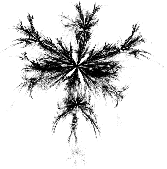
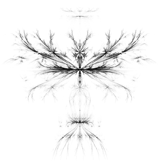
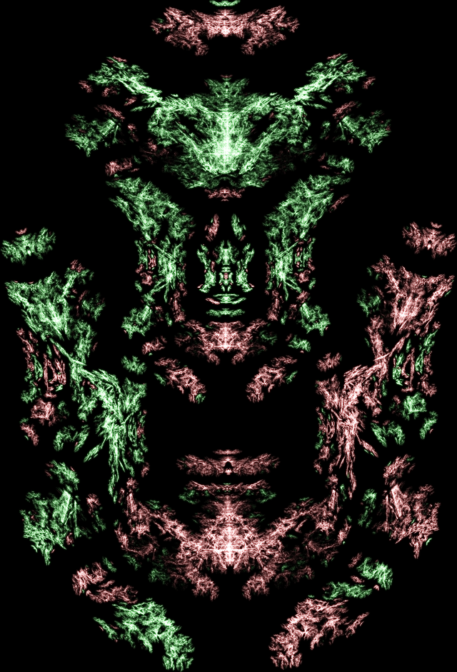
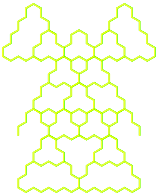
What's great about these structures is that they are still fractals. They may look spazzy and some of them may remind you of Vash the Stampede's plant mode arm, but they possess self-similarity throughout. For example, why do the arms of the nest look like that?

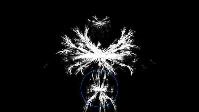
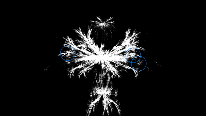
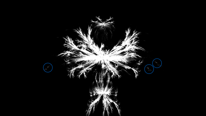
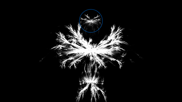
It's because the nest as a whole looks like that. And notice that as the big bird flies in from below to explode into the nest, the little birds all around the nest follow along (because adults know best) and explode into their own little nests, and so on, producing the distinctive infinitary echela of simultaneously exploding dinosaur progeny. And notice that the big bird itself is a version of the entire figure. Now, as for the hat, who knows.

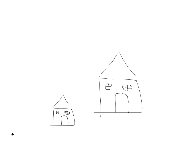
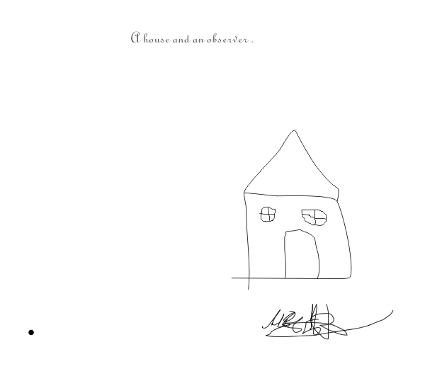
The chaos game is an algorithm that we use for the sake of computational convenience. The "real" algorithm doesn't randomly pick among the vertices, it takes every point toward every observer at each step. And it's actually easy to see how the self-similarity of the algorithm comes about. Look here at a house and an observer:

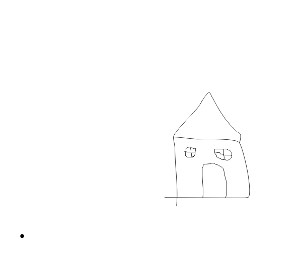
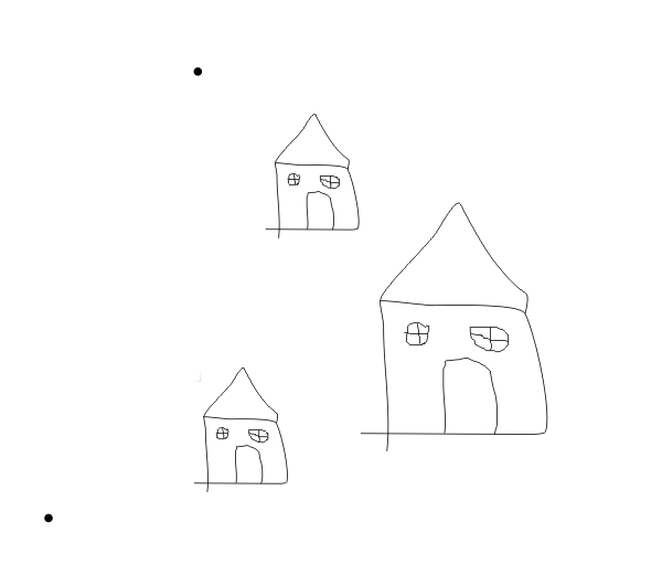
If we run one step of the "real" algorithm, we get this. Something interesting here is that there is no difference between what the observer sees in either case. The little house is exactly blocking his or her view of the bigger house, like an inescapable mathematical version of a really tall person sitting in front of you at a theatre (formally we would say the houses are cosyzygous). If we start with two observers, we get this then this.

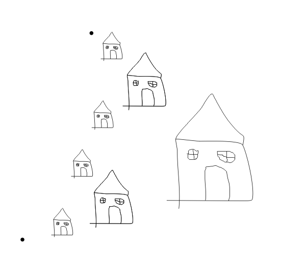
Another way of thinking about it is that the resulting figure is precisely the figure that all observers "agree on":

Because running the full algorithm on the entire figure does nothing. I.e. the figure is the fixed point of the algorithm. This automagic consensusing bonks my head and seems to me to carry a particular philosophical undertone... over which I shalln't digress.

Mathematically, it appears our chaos game shennaneganery as a whole falls under the contraction mapping principle. Tersely complicated explanations of inconfusably simple things not withstanding, I know me some topology but not enough to understand the bigger picture of what's going on.

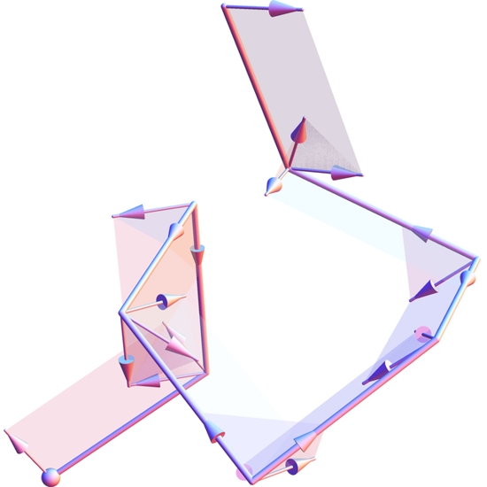
On the subject of hats, when going from 2D L-systems to 3D L-systems I had to put a hat on the turtle and also give it the ability to do backflips and taco rolls:

Even wearing Mugen's shoes. Wow. Unfortunately, as epic as this is, with our current technology we're limited to e.g. representing the turtle's hat with an abstraction called a "vector", which certainly doesn't connote the same social status or sophistication. Still it's enough for some 3D L-systems, such as this version of the arrowhead construction:

Module[{options = {
     Axiom -> None, Rules -> {}, Iterations -> 1, Definitions -> {},
     DrawStyle -> {}, HatStyle -> {}, Primitive -> Tube, TraceHat -> False,
     HatWorldplaneStyle -> Directive[EdgeForm[None], Opacity[.2]],
     HatPrimitive -> Composition[Arrow, Tube], Angle -> 2. Pi/6,
     RandomStuff -> Sphere[{0, 0, 0}, .05]}},

  SetAttributes[Draw, Orderless];

  Draw[commands : {Except[_Rule | _RuleDelayed] ..},
    rules : {(_Rule | _RuleDelayed) ..}, rest___] := Draw[Axiom -> commands, Rules -> rules, rest];                
  Draw[rules : {(_Rule | _RuleDelayed) ..}, rest___] := Draw[Rules -> rules, rest];
  Draw[commands : {Except[_Rule | _RuleDelayed] ..}, rest___] := Draw[Axiom -> commands, rest];
  Draw[opts : OptionsPattern[Join[Options[Graphics3D], options]]] :=
   Module[{commands, reshape, states, points, hatTrace, hatWorldplane,
     forwardP, leftP, frontflipP, tacoleftP, flipoutP, pushI, popI, definitionsI},

    (*basic parameterized state transfer functions*)
    forwardP[p_][{z_, face_, hat_}] := {z + p face, face, hat};
    leftP[p_][{z_, face_, hat_}] := {z, RotationTransform[p, hat][face], hat};
    tacoleftP[p_][{z_, face_, hat_}] := {z, face, RotationTransform[p, face][hat]};
    frontflipP[p_][{z_, face_, hat_}] := Module[{rot},
      rot = RotationTransform[p, Cross[hat, face]];
      {z, rot[face], rot[hat]}];
    flipoutP[p1_, p2_] := Composition[frontflipP[-p2], tacoleftP[-p1]];

    (*general function. fit elements of l1 into structure of l2*)
    reshape[l1_, l2_] := Module[{i = 1, length = Length[l1]},
      Map[l1[[Mod[i++, length, 1]]] &, l2, {-1}]];

    (*LIFO stack*)
    {pushI, popI} = Module[{stack = {}},
      {(AppendTo[stack, #]; #) &,
       Module[{val = Last[stack]},
         stack = Most[stack];
         val] &}];

    With[{vars = First /@ options},
     Module[vars, vars = OptionValue[vars];

 If[Axiom === None && Rules =!= {}, Axiom = Rules[[1, 1]]];(*default axiom*)
      Axiom = Flatten[{Axiom}];(*normalize to list/directive*)
      {DrawStyle, HatStyle, HatWorldplaneStyle} = Directive /@ {DrawStyle, HatStyle, HatWorldplaneStyle};

      Definitions = Join[Definitions, {
         F -> forward, B -> backward, L -> left, R -> right, FO -> flipout, FO[p_] :> flipout[p],
         FF -> frontflip, BF -> backflip, TL -> tacoleft, TR -> tacoright}];

      definitionsI = {
        forward[p_] :> forwardP[p], backward[p_] :> forwardP[-p], left[p_] :> leftP[p],
        right[p_] :> leftP[-p], tacoleft[p_] :> tacoleftP[-p], tacoright[p_] :> tacoleftP[p],
        frontflip[p_] :> frontflipP[p], backflip[p_] :> frontflipP[-p], forward -> forwardP[1],
        backward -> forwardP[-1], left -> leftP[Angle], right -> leftP[-Angle], tacoleft -> tacoleftP[-Angle],
        tacoright -> tacoleftP[Angle], frontflip -> frontflipP[Angle], backflip -> frontflipP[-Angle],
        flipout -> flipoutP[Angle, Angle], flipout[p1_] :> flipoutP[p1, Angle],
        flipout[p1_, p2_] :> flipoutP[p1, p2], push -> pushI,
        pop -> Sequence[popI, Identity](*preadjustment for reshape*)};

      (*note no memoization. if you try, keep in mind case of RuleDelayed*)
      commands = Nest[Flatten[Replace[#, Rules, {1}]] &, Axiom, Iterations];
      commands = Flatten[((# /. Definitions) /. definitionsI) & /@ commands];
      states = ComposeList[commands, N@{{0, 0, 0}, {0, 1, 0}, {0, 0, 1}}];

      points = reshape[First /@ states, Split[popI === # & /@ Join[{0}, commands]]];(*pop is turtle teleportation*)
      points = Composition[First /@ # &, Split] /@ points;(*delete duplicate points*)

      Graphics3D[{
        {RandomStuff /. None -> {}, {DrawStyle, Primitive[points]}},
        If[TraceHat,
         hatTrace = {#1, #1 + 2 #3/5} & @@@ states;
         hatTrace = First /@ Split[hatTrace];(*delete duplicate hats*)

         hatWorldplane = Polygon[{#1, #2, #4, #3} & @@ Flatten[#, 1]] & /@ Partition[hatTrace, 2, 1];
         {{HatStyle, HatPrimitive[hatTrace]}, {HatWorldplaneStyle, hatWorldplane}}, {}]},
       Quiet@FilterRules[{opts}, Options[Graphics3D]], Boxed -> False]]]]];

Draw[
 {X, push, BF, L, X, R, R, X, pop, R, X, L, TL, L, X, R, F},
 {F -> {F, BF, push, L, X, R, R, X, pop, R, X, L, L, X, R, F},
  X -> {F, BF, push, L, F, R, R, R, F, pop, R, F, L, L, F, R, F}},
 Iterations -> 3, DrawStyle -> {Opacity[.65], Glow[Darker[Red, 2/3]]},
 Definitions -> {X -> Identity}, Angle -> Pi/8]

Whoops. Accidentally X-rayed my heart. Or was that this one? In any case, this is the 3D Sierpinski arrowhead curve. It might not look very 3D, but technically it's 3D because it's made out of a tube instead of a line. All joking aside, try as I might I wasn't able to figure out the construction for the 3D arrowhead curve, sadface.

And though this a crushing defeat, we here at the Sierpinski triangle page are stalwart folk for whom such failure is but a rare trigger of recidivistic saccades to our respective vices, for in the characteristic case we amene our fibrile egos by way of the platitudinous homily that what doesn't kill you makes you stronger. In the process of trying to figure out the 3D arrowhead I ended up making an easy-to-use flexible L-system program.

True story, when I woke up this morning I could have sworn my body was contorting into different LOGO curves, in the hope of trial-and-erroring the arrowhead construction. It was like that dream scene in Fight Club, except instead of a girl it was a LOGO curve. Definitely one of the more Freudiologically-awkward memories I'm going to have to carry around for the rest of my life.

proc[img1_, cf_: ColorData[1], mode_: None, blur_: 8] :=
  Module[{img, components, rank, largest, colored},
   img = RemoveAlphaChannel[ColorNegate@ColorConvert[img1, "Grayscale"]];
   components = MorphologicalComponents[img];

   Module[{measurements, sorted},
    measurements = ComponentMeasurements[components, "Count"];
    sorted = First /@ Reverse@SortBy[measurements, Last];
    rank[label_] := (rank[label] = Position[sorted, label][[1, 1]])];

   colored = Colorize[components, ColorFunction -> (cf[rank[#]] &), ColorFunctionScaling -> False];
   If[mode == "Angelic", colored = ImageMultiply[img, colored]];
   ColorNegate[ImageMultiply[ColorNegate[img], Blur[#, blur] &@ColorNegate[colored]]] // ImageAdjust];

(**)im = Draw[Iterations -> 17, {F -> {B, left[.020944], B}, B -> {L, F}}, RandomStuff -> None,
    Angle -> Pi/5, ImageSize -> 1280, ViewPoint -> {0, 0, Infinity}] // Rasterize;

GradientFilter[im, 5] // ColorNegate // proc[#, Blue &] & // ColorNegate // ImageResize[#, Scaled[1/2]] &

(**)Draw[{A -> {B, L, B}, B -> {A, R, A}}, Primitive -> (Rotate[Line[#], -Pi/24, {0, 0, 1}] &),
 Iterations -> 13, Angle -> 7 Pi/12, Definitions -> {B -> forward, A -> forward},
 DrawStyle -> Opacity[.5], RandomStuff -> None, ViewPoint -> {0, 0, Infinity}]

(**)Draw[Iterations -> 9, {A -> {B, L, B}, B -> {A, R, A}}, Definitions -> {B -> forward, A -> forward},
   RandomStuff -> {Transparent, Sphere[{0, 0, 0}, .05]}, DrawStyle -> {Opacity[.8], Yellow, Glow[Green]},
   ViewPoint -> {0, 0, Infinity}]

(**)d = Draw[{swirl -> ConstantArray[{BF, F, BF, swirl, FO[Pi/12]}, 5]}, DrawStyle -> Opacity[.9], RandomStuff -> None,
    Primitive -> (Line[First@#,
      VertexColors -> (Darker[#, 1/8] & /@ ColorData["AvocadoColors"] /@ Range[0., 1, 1/(Length[First[#]] - 1)])] &),
    Definitions -> {swirl -> backward}, Iterations -> 6, ImageSize -> 2 1280, Method -> {"ShrinkWrap" -> True},
    Background -> Lighter[LightGray, 7/12]] // Rasterize;

d // ImageResize[#, Scaled[1/4]] & // ImageReflect[#, Top -> Bottom] & // ImagePad[#, 2, Lighter[LightGray, 7/12]] &

(**)Draw[Iterations -> 8, {F :> {F, flipout[.2 RandomReal[], Pi RandomReal[]], F}}]

(**)h = Draw[{R -> {B, R, R, R, F}}, Iterations -> 8, Primitive -> Line, RandomStuff -> None,
    Angle -> 1907/2048, ImageSize -> 2 1280, ViewPoint -> {0, 0, Infinity}] // Rasterize;

proc[h // ImageAdjust, Yellow &, "Anglic", 13] // ImageResize[#, Scaled[1/4]] &

(**)diff = ImageDifference @@ Table[
   Draw[{arc, F, arc}, {F -> {F, F, arc, F, arc, F, arc, F, F}}, Primitive -> (Tube[#, .115] &), Angle -> Pi/6,
     Definitions -> {F -> forward[6], arc -> Flatten[Table[{forward[.1], backflip[.899 .1047], right[1/4 .1047]}, {160}]]},
     Iterations -> 2, DrawStyle -> color, RandomStuff -> None, Lighting -> "Neutral", Method -> {"ShrinkWrap" -> True},
     ViewPoint -> {3, -0.25, -1.5}, ViewVertical -> {0.56, -0.66, -0.7}, ImageSize -> 2 1280] // Rasterize,
   {color, {LightGray, White}}];

diff // ColorNegate // ImageAdjust // ImageResize[#, Scaled[1/4]] &

What makes this program great is that even just for 2D L-systems, the 3D perspective makes things more intuitive. The arrowhead problem also demanded debugging features such as keeping track of the turtle's orientation, a definite necessity because of the enormous degrees of freedom that geometric L-systems possess.

To give you an idea of this freedom, all of the items in this table are the same exact L-system at the same exact power. The only difference between them is the base angle specified. (By the way, notice Voltron. This is how you know L-systems are Turing complete.) If you take a couple of these to higher powers you get these images (11th and 13th iterations). It's interesting to wonder what some of these might look like at say the thousandth or billionth iteration. Or even, the millionth.

Sidenote. You may have noticed that I never really explained what L-systems are. In fact what I do and don't explain on this page is pretty much completely arbitrary, largely to annoy people who are already familiar with all of this stuff. "Why aren't you mentioning IFS" I hear them crying. Hilarious. But if you've used Mathematica you know that it's well-suited for replacement schemes such as L-systems in a way that is difficult to convey in the context of other languages. Take a look at a simple function definition in Mathematica:

add[a_, b_] := a + b

add[_, _] := 1

What this is saying is: Whenever something matching the pattern add[a_, b_] is found, replace it by a + b. In other words, function application is a special case of pattern matching. Those _ characters are the analogue of the regex . character, the Kleene proton. So a_ means "match any single thing, and call it a". You can in fact do this, which will make the 'function' return 1 when it is passed any two things, as well as use more involved patterns.

I point this out because it can be difficult to appreciate the fundamental straightforwardness of the Mathematica language, I think even for people who have used it for a while. And especially if you're coming to Mathematica from more mainstream languages where the idea of function application being a special case of something more general would be considered some kind of unreachable koan.

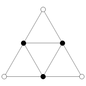
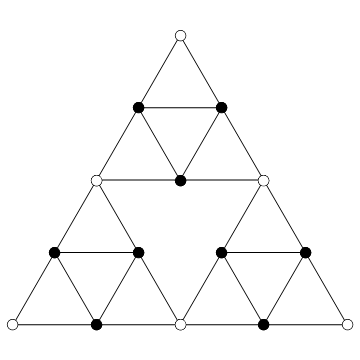
The arrowhead isn't the only L-system that can create the Sierpinski figure. More likely there are an infinite number of distinct L-systems that form the Sierpinski triangle in the limit. When we were fiddling with the Sierpinski triangle as a graph, you may have noticed that the zig zag and criss cross had recursive structure:

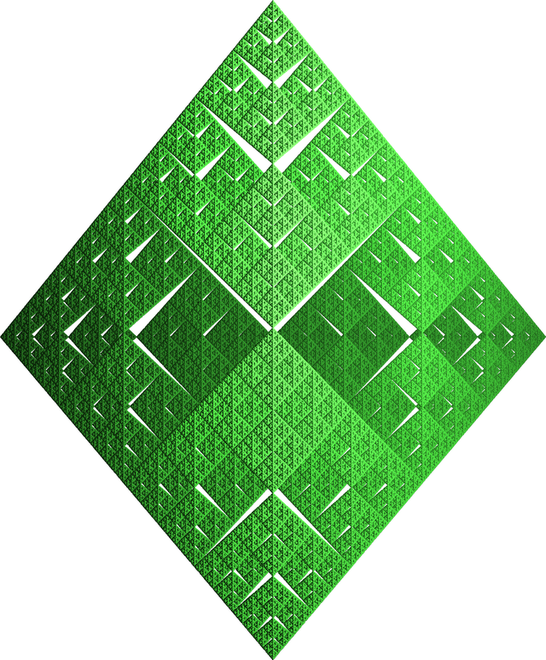
With[{v = 5},
  axiom = Polygon[{Cos[#], Sin[#]} & /@ (2 Pi Range[v]/v)]];

next[prev_] := prev /. Polygon[pts_] :>
    (Polygon[ScalingTransform[1/2 {1, 1}, #][pts]] & /@ pts);

draw[n_] := Module[{edges},
   edges = Flatten@Nest[next, N@axiom, n] /. Polygon[pts_] :>
      Sequence @@ UndirectedEdge @@@ Partition[pts, 2, 1, 1];

   Graph[edges, VertexCoordinates -> VertexList[Graph[edges]],
    VertexSize -> .25]];

draw[2]
GraphPlot3D[draw[2]]

axiom = Polygon[{{0, 0}, {1, Sqrt[3]}/2, {1, 0}}];

next[prev_] := prev /. Polygon[{p1_, p2_, p3_}] :> {
     Polygon[{p1, (p1 + p2)/2, (p1 + p3)/2}],
     Polygon[{p2, (p2 + p3)/2, (p1 + p2)/2}],
     Polygon[{p3, (p1 + p3)/2, (p2 + p3)/2}]};

draw[n_] := Module[{edges},
   edges = Flatten@Nest[next, N@axiom, n] /. Polygon[pts_] :>
      Sequence @@ UndirectedEdge @@@ Partition[pts, 2, 1, 1];

   Graph[edges, VertexCoordinates -> VertexList[Graph[edges]],
    VertexSize -> .25]];

g = draw[2];
cycle = RandomChoice[{FindHamiltonianCycle, FindEulerianCycle}][g][[1]];

Animate[
 HighlightGraph[g, Graph[cycle[[1 ;; n]]],
  EdgeShapeFunction -> (Line[#1] &),
  VertexShapeFunction -> None,
  GraphHighlightStyle -> "DehighlightHide"],
 {n, 1, Length[cycle], 1}, AnimationRate -> 1]

We can find these paths for the 3D Sierpinski graph as well, though not necessarily. In fact all along we could have been grapherizing a lot of our stuff, even things like the different distance functions. My point here however is that we may be able to reverse-engineer an L-system from these structures. And it might not actually be hard at all. It does have the down side however of sounding really boring, so on to nonboringer pastures we skidaddle-prance.

Since cellular automata often have the 'world' array joined at the ends, it makes sense to think of their evolution as being on a cylinder:

draw[array_, options___] := Module[
   {interval, topinterval, width, height, f, coords},
   {height, width} = Dimensions[array];
   interval = 2. Pi/width;
   topinterval = 2. Pi (1 + interval)/width;
   coords = Position[array, 1];

   f[{x_, r_}] := Rotate[Translate[
      Cuboid[-#, #] &[.5 topinterval {1, 1, 1}],
      {1, 0, -interval x}], interval r, {0, 0, 1}(*;{1,0,0}*), {0, 0, 0}];

   Graphics3D[{{Lighter[LightBlue], Opacity[.5],
      Sphere[{0, 0, -interval height/2}, .5]},
     EdgeForm[None], White, f /@ coords}, options, Boxed -> False]];

draw[CellularAutomaton[22,
  ConstantArray[0, 500]~ReplacePart~{1 -> 1, 251 -> 1}, 125],
 Lighting -> "Neutral"]

draw2[im_Image, options___] := draw2[ImageData[ColorConvert[im, "RGB"]], options];
draw2[array_, options___] := Module[
   {interval, width, height, f, cubes, coords},
   {height, width} = Dimensions[array][[{1, 2}]];
   interval = 2. Pi/width;
   coords = Position[array, p_ /; p != {0, 0, 0}, {2}];

   f[{x_, r_}] := Rotate[Translate[
      Cuboid[-#, #] &[.5 interval {1, 1, 1}],
      {1, 0, -interval x}], interval r, {0, 0, 1}, {0, 0, 0}];

   cubes = MapThread[{RGBColor @@ #1, f[#2]} &,
     {array[[##]] & @@@ coords, coords}];

   Graphics3D[{{Lighter[LightBlue], Opacity[.5],
      Sphere[{0, 0, -interval height/2}, .5]},
     EdgeForm[None], cubes}, options, Boxed -> False]];

(*this rule from "http://web.cecs.pdx.edu/~mm/evca-review.pdf"*)
rules = Thread[Tuples[{0, 1}, {7}] ->
    IntegerDigits[FromDigits["0504058705000f77037755837bffb77f", 16], 2, 128]];

arr = FixedPointList[CellularAutomaton[rules], RandomInteger[1, 600]];
arrEdge = ArrayPlot[arr, PixelConstrained -> 1, Frame -> False] // EdgeDetect // ImageData;

(*ad hoc coloring, originally intended for particle animation*)
pat1 = {{_, _, _, _, _}, {_, 1, 0, 0, 1}, {_, _, _, _, _}};
pat2 = {{_, 1, _, _, _}, {_, _, 1, _, _}, {_, _, _, 1, _}};
pat3 = {{_, _, _, _, _}, {_, 1, 1, 1, _}, {_, _, _, _, _}};
(f[#1 | Reverse /@ #1, _] = #2) & @@@
  {_ -> {0, 0, 0}, pat1 -> {1, 0, 0}, pat2 -> {0, 1, 0}, pat3 -> {0, 0, 1}};

(*see also ImageFilter, ImageConvolve, a million other things*)
colored = CellularAutomaton[{f, {}, {1, 2}}, arrEdge];

Image[colored]
draw2[colored, Lighting -> "Neutral"]

This is Rule 22 with two initial black squares. It's a cylindrical mapping of this. The sphere in the center is an homage to the Sega Saturn. Long live Sega Saturn, long live Dreamcast. Neo Geo forever. This is a different projection of the same thing, which might actually be easier to comprehend than the cylindrical projection.

And a plot of a range-7 automaton, described in this paper, that was evolutionarily engineered to discriminate between majority-white and majority-black initial conditions. And a particle plot oNEKO!!! Ka-wa-ii. My hope is the image of this dark hieroglyphic cat infests your dreams with nightmares so mindbendingly horrid your perception of reality and fantasy becomes forever warped. Whoops did I say that out loud. See also my Cellular Automata program.

Of course, there are automata whose evolutions are properly three-dimensional, like these quadrilateral versions of Rule 22:

draw[block_, options___] := Graphics3D[
   {EdgeForm[Gray], Cuboid /@ Position[block, 1]},
   options, ViewVertical -> {-1, 0, 0}, Boxed -> False];

draw[CellularAutomaton[{
115792089237316195423570985008687907853269984665640564039476030751986839257106
  , 2, {1, 1}}, {{{1}}, 0}, 31],
 Lighting -> "Neutral"]

(**)
grids = Partition[#, 3] & /@ Tuples[{1, 0}, {9}];
rule = IntegerDigits[#, 2, 512] &@
   115792089237316195423570985008687907853269984665640564039476030751986839257106;

Dynamic[FromDigits[rule, 2]]
Dynamic[draw[CellularAutomaton[{FromDigits[rule, 2], 2, {1, 1}}, {{{1}}, 0}, 31]]]

With[{plot = Function[c, Magnify[ArrayPlot[#1, FrameStyle -> c], 1/6]]},
 Grid[Partition[#, 32], Spacings -> {.1, .1}] &@
  MapIndexed[
   Toggler[Dynamic[rule[[First@#2]]],
     {0 -> plot[LightGray], 1 -> plot[Red]}] &,
   grids]]

(**)
z = Import["http://upload.wikimedia.org/wikipedia/commons/thumb/e/e0/Game_of_life_glider_gun.svg/610px-Game_of_life_glider_gun.svg.png"];
z = ImageData[ImageResize[z, Scaled[1/16], Resampling -> "Nearest"] // Binarize // ColorNegate];
Image[z] // Magnify

With[{f = Switch[
     {#[[2, 2]], Total[#, 2] - #[[2, 2]]},
     {_, 3} | {1, 2}, 1, _, 0] &},

 draw[CellularAutomaton[{f, {}, {1, 1}}, {z, 0}, 100]]]

An actual 3D automaton whose evolution would be 4-dimensional:

draw[block_, options___] := Graphics3D[
   {EdgeForm[Darker[Gray]], Cuboid /@ Position[block, 1]},
   options, ViewVertical -> {-1, 0, 0}, Boxed -> False];

f[block_, _] := Switch[
   {block[[2, 2, 2]], Total[block, 3] - block[[2, 2, 2]]},
   {_, 4}(*|{1,2}*), 1, _, 0];

evol = CellularAutomaton[{f, {}, {1, 1, 1}},
   {{{{1, 1}, {1, 1}(*,{1,1},{1,1}*)}}, 0}, 15];

ListAnimate[
 draw[#, Lighting -> "Neutral", ImageSize -> 400 {1, 1}] & /@ evol]

draw[block_, options___] := Graphics3D[{
    EdgeForm[None],(*Opacity[.8],*)
    Cuboid /@ Position[block, 1],
    Black, Cuboid /@ Position[block, 2]},
   options, Lighting -> "Neutral", Boxed -> False];

f[block_, _] := Switch[
   {block[[2, 2, 2]], Total[block, 3] - block[[2, 2, 2]]},
   {_, 4}, 1, {0, 3}, 2, _, 0];

evol = CellularAutomaton[{f, {}, {1, 1, 1}},
   {CrossMatrix[1 {1, 1, 1}]~BitXor~1, 0}, 25];

(*can be flashy*)
(*ListAnimate[draw[#,ViewPoint->Top,ImageSize->400 {1,1}]&/@evol]*)

draw[Last[evol],
   ImageSize -> 2 1280, ViewPoint -> 2 {1, 1, 1},
   Lighting -> {{"Point", Yellow, Scaled[{1, 1, 1}], 5}},
   Method -> {"ShrinkWrap" -> True}] //
  Rasterize // ImageResize[#, Scaled[1/4]] &

And just so we're all clear, time isn't "the fourth dimension." That statement is the conceptual version of eating bagels without cream cheese, namely a manifestation of meaniglessness.

If you have Mathematica 9 (must be nice), its Image3D functionality is perfect for these 3Dified cellular automata. And speaking of grid thingies, let's not forget our unexpectedly-glorious matrix replacement scheme:

(**)
Begin["mmx`"];

matrixInput3D1[Dynamic[tensor_], Dynamic[color_], options___] :=
  Dynamic@Module[{grid},
    grid = Position[ArrayPad[tensor, {0, -1}], _?IntegerQ];

    EventHandler[#, {"MouseDown", 2} :> {}] &@
       Graphics3D[{#, Transparent, EdgeForm[LightGray], Cuboid /@ grid},
        options,(*Method->{"ShrinkWrap"->True},*)Boxed -> False] &@

     Array[With[{loc := tensor[[##]]},
        Mouseover[
         (**){Style[#, Darker[color, .65]] &@
           Text[Dynamic[loc /. 0 -> Style[0, Opacity[.5]]], {##}],
          Opacity[loc /. {0 -> .1, 1 -> .3}], Sphere[{##}, .2]},
         (**){Text[EventHandler[Checkbox[Dynamic[loc], {0, 1}],
            {"MouseDown", 2} :> (loc = 0)], {##}],
          Opacity[.01], Sphere[{##}, .2]}]] &,
      Dimensions[tensor]]];

matrixInput3D2[Dynamic[tensor_], Dynamic[rules_], Dynamic[color_], options___] :=
  Dynamic@DynamicModule[{grid},
    grid = Flatten[Array[List, Dimensions[ArrayPad[tensor, {0, -1}]]], 2];

    EventHandler[#, {"MouseDown", 2} :> {}] &@
       Graphics3D[{#, Transparent, EdgeForm[LightGray], Cuboid /@ grid},
        options,(*Method->{"ShrinkWrap"->True},*)Boxed -> False] &@

     Array[With[{loc := tensor[[##]]},
        With[{display = Tooltip[Panel[#, FrameMargins -> None],
             Column[{loc /. rules /. {Reverse -> "R", Transpose -> "T",
                 Composition -> List, Verbatim[Slot][_] :> "m"},
               "", "Click to cycle", "Right-click to zero"}],
             TooltipDelay -> .6] &},

         Mouseover[
          (**){Style[#, Darker[color, .65]] &@
            Text[Dynamic[loc /. 0 -> Style[0, Opacity[.5]]], {##}],
           Opacity[loc /. {0 -> .1, _ -> .3}], Sphere[{##}, .2]},
          (**){Text[EventHandler[
             display[
              Toggler(*PopupMenu*)[Dynamic[loc], First /@ rules,
               ImageSize -> Automatic]
              ],
             {"MouseDown", 2} :> (loc = 0)], {##}],
           Opacity[.01], Sphere[{##}, .2]}]]] &,
      Dimensions[tensor]]];

bg = White;
dims = # -> If[# > 2, Style[#, Red], #] & /@ Range[5];

rotations = Flatten@Outer[Function[{o, dir},
     Composition[Transpose[#, o] &, dir /@ # &, Transpose[#, o] &]],
    {{1, 2, 3}, {3, 2, 1}, {2, 1, 3}},
    {Composition[Transpose, Reverse],
     Composition[Reverse, Transpose],
     Reverse, Transpose}, 1];

rotations = MapIndexed["S" @@ #2 -> #1 &, rotations];
defaultRules = Join[{0 -> (0 # &), 1 -> (# &)}, rotations];

iterate[matrix0_, matrixT_, rules_, power_] :=
  Nest[Function[prev,
    ArrayFlatten[Map[#[prev] &,
      Replace[matrixT, rules, {3}], {3}], 3]],
   matrix0, power];

randomMatrix[dimensions_, source_] := With[
   {rv := RandomVariate[ZipfDistribution[Length[source], 1]]},
   Array[source[[rv]] &, dimensions]];

With[{HiPrint := Function[viewpoint,
    With[{pow = power},
     CellPrint[ExpressionCell[
       Defer[
        powzerz = pow;
        With[{objects = Translate[primitive,
            Replace[Position[iterate[
               matrix0 /. 0 matrix0 -> {{{1}}},
               matrixT /. 0 matrixT -> {{{1}}},
               rules, powzerz], If[negativeSpace, 0, 1]],
             {} -> {1, 1, 1}]]},
         ImageResize[Rasterize[#], Scaled[1/4]] &@
          Defer[Graphics3D][{color, Opacity[opacity],
            Glow[glow], Specularity[specularity],
            EdgeForm[{Opacity[opacity], Darker[color, 4 .15]}], objects},
           Lighting -> "Neutral", Method -> {"ShrinkWrap" -> True},
           ImageSize -> {Automatic, 4 732}, Boxed -> False,
           ViewPoint -> viewpoint, ViewVertical -> vv,
           Background -> background]]],
       "Input"]]]],

  printMatrices := Function[
    CellPrint[ExpressionCell[DynamicModule[{
        mtx0 = matrix0, mtxT = matrixT, mtx0o = matrix0, mtxTo = matrixT,
        clr = color, opc = opacity, ns = negativeSpace, pow = power, rls = rules,
        prm = primitive, iter = iterate, bg = background, vp1 = vp, vv1 = vv},

       With[{
         btn = Button[DynamicWrapper["print data",

            If[mtx0 =!= mtx0o || mtxT =!= mtxTo, mtx0 = mtx0o; mtxT = mtxTo]],
           Print[Grid[{
              {"kernel matrix", MatrixForm[mtx0o]},
              {"transformation matrix", MatrixForm[mtxTo]},
              {"rules", rls}, {"power", pow}}]]],
         mtx0c = matrixInput3D1[Dynamic[mtx0], Dynamic[clr],
           SphericalRegion -> True, ImageSize -> Small,
           Background -> Lighter[bg, .8],
           ViewPoint -> Dynamic[vp1], ViewVertical -> Dynamic[vv1]],
         mtxTc = matrixInput3D2[Dynamic[mtxT], Dynamic[rls], Dynamic[clr],
           SphericalRegion -> True, ImageSize -> Small,
           Background -> Lighter[bg, .8],
           ViewPoint -> Dynamic[vp1], ViewVertical -> Dynamic[vv1]],
         g3d = With[{objects = Translate[prm,
              Replace[Position[iter[
                 mtx0 /. 0 mtx0 -> {{{1}}},
                 mtxT /. 0 mtxT -> {{{1}}},
                 rls, pow], If[ns, 0, 1]],
               {} -> {1, 1, 1}]]},
           Graphics3D[{
             EdgeForm[{Opacity[opc], Darker[clr, 4 .15]}],
             clr, Opacity[opc], objects},
            ImageSize -> Small, Boxed -> False, SphericalRegion -> True,
            ViewPoint -> Dynamic[vp1], ViewVertical -> Dynamic[vv1],
            Lighting -> "Neutral", Background -> bg]]},

        Panel[Grid[{
           {Panel[Placeholder["name"]], SpanFromLeft, btn},
           {mtx0c, mtxTc, g3d}}]]]]]]],

  (* controls *)
  dim0C = Control[{{dim0, 1, ""}, dims, ControlType -> PopupMenu}],
  dimTC = Control[{{dimT, 2, ""}, dims, ControlType -> PopupMenu}],
  matrix0C = matrixInput3D1[Dynamic[matrix0], Dynamic[color],
    SphericalRegion -> True, ImageSize -> Dynamic[imgSize1],
    Background -> Dynamic[Lighter[background, .8]],
    ViewPoint -> Dynamic[vp], ViewVertical -> Dynamic[vv]],
  matrixTC = matrixInput3D2[Dynamic[matrixT], Dynamic[rules], Dynamic[color],
    SphericalRegion -> True, ImageSize -> Dynamic[imgSize2],
    Background -> Dynamic[Lighter[background, .8]],
    ViewPoint -> Dynamic[vp], ViewVertical -> Dynamic[vv]],
  rulesC = Pane[Style[#, 10], {400, 200}, Scrollbars -> Automatic] &@
    Control[{{rules, defaultRules, ""},
      InputField, Background -> Dynamic[Lighter[background, .65]],
      FieldSize -> {50, {0., Infinity}}}],
  colorC =
   Control[{{color, RGBColor[.15, .6, 1], "color"}, ColorSlider}],
  backgroundC = Row[{"background   ", Framed[
      ColorSlider[Dynamic[background, (bg = background = #) &],
       AppearanceElements -> "Swatch"],
      FrameStyle -> Gray], " ",
     ColorSlider[Dynamic[background, (bg = background = #) &],
      AppearanceElements -> "Spectrum", ImageSize -> Small]}],
  opacityC = Control@{{opacity, 1, "opacity"}, 0, 1, ImageSize -> Small},
  glowC = Control[{{glow, Black, "glow"}, ColorSlider}],
  specC = Control[{{specularity, Black, "specularity"}, ColorSlider, ImageSize -> Small}],
  primC = Control[{{primitive, Scale[Cuboid[],.99999], "primitive"},
     # -> Graphics3D[{color, #}, Boxed -> False, ImageSize -> 20] & /@
      {{PointSize[0], Point[{0., 0., 0.}]}, Sphere[{0., 0., 0.}, .5],
       {EdgeForm[None], Scale[Cuboid[],.99999]}, Scale[Cuboid[],.99999]}, SetterBar}],
  powerC = Control[{{power, 1, "power"}, 0, 5, 1, Appearance -> "Labeled"}],
  nsC = Control[{{negativeSpace, False,
      Tooltip["negative", "negative space",
       TooltipDelay -> .4]}, {False, True}}]
  },

 (*control layout*)
 With[{controls :=
    Row[{
      Column[{
        Row[{dim0C, "   |", dimTC}],
        Row[{"    ", matrix0C, "  ", matrixTC}]}], Spacer[40],
      Column[{
        OpenerView[{"Rules", rulesC}],
        OpenerView[{"Style",
          Column[{
            Row[{
              Column[{colorC, backgroundC}], Spacer[40],
              Column[{glowC, specC}]}],
            Row[{opacityC, Spacer[20], nsC, Spacer[20], primC}]}]}],
        powerC}]}],

   bookmarks := {
     Overscript["Random kernel matrix", ""] :>
       (matrix0 = randomMatrix[Dimensions[matrix0], {0, 1}]),
     "Random transformation matrix" :>
       (matrixT = randomMatrix[Dimensions[matrixT], First /@ defaultRules]),
     "Random both" :> (
       matrix0 = randomMatrix[Dimensions[matrix0], {0, 1}];
       matrixT = randomMatrix[Dimensions[matrixT], First /@ defaultRules]),

     Overscript["Clear kernel matrix", ""] :> (matrix0 = 0 matrix0),
     "Clear transformation matrix" :> (matrixT = 0 matrixT),
     "Clear both" :> ({matrix0, matrixT} = 0 {matrix0, matrixT}),

     Overscript["Invert kernel matrix", ""] :> (matrix0 = BitXor[matrix0, 1]),
     "Invert transformation matrix" :> (matrixT = Replace[matrixT, {0 -> 1, _ -> 0}, {3}]),

     Overscript["Print matrices", ""] :> printMatrices[],

     Overscript["HiPrint", ""] :> HiPrint[vp],
     "HiPrint Far" :> HiPrint[1000 vp]}},

  Panel[#, Background -> Dynamic[bg]] &@
   Manipulate[Module[{g3d, side},

     If[dim0 {1, 1, 1} =!= Dimensions[matrix0], matrix0 = PadRight[matrix0, dim0 {1, 1, 1}]];
     If[dimT {1, 1, 1} =!= Dimensions[matrixT], matrixT = PadRight[matrixT, dimT {1, 1, 1}]];
     If[bg =!= background, bg = background];

     Module[{matrixP},(*remove rules from matrix that no longer exist*)
      matrixP = Map[Function[a, If[a === Replace[a, rules], rules[[1, 1]], a]], matrixT, {3}];
      If[matrixT =!= matrixP, matrixT = matrixP]];

     g3d = With[{objects = Translate[primitive,
          Replace[Position[iterate[
             matrix0 /. 0 matrix0 -> {{{1}}},
             matrixT /. 0 matrixT -> {{{1}}},
             rules, power], If[negativeSpace, 0, 1]],
           {} -> {1, 1, 1}]]},
       Graphics3D[{
         Dynamic[EdgeForm[{Opacity[opacity], Darker[color, 4 .15]}]],
         Dynamic[color], Dynamic[Opacity[opacity]], Dynamic[Glow[glow]],
         Dynamic[Specularity[specularity]], objects},
        ImageSize -> {{300, Large}, {300, Large}},
        Lighting -> "Neutral", Background -> Dynamic[background]]];

     side = Map[Function[vp1,
        Tooltip[#, ViewPoint -> vp1, TooltipDelay -> .3] &@

           EventHandler[#,
            "MouseDown" :> (vp = vp1 /. Infinity -> 4; vv = {0, 0, 1})] &@
         Framed[Deploy[
           Show[g3d, ViewPoint -> vp1, ImageSize -> Small, Boxed -> False]],
          FrameStyle -> Gray, Background -> Dynamic[background]]],
       Permutations[{Infinity, 0, 0}]];

     Row[{Column[side,(*Dividers->All,*)FrameStyle -> Gray],
       Show[g3d, Boxed -> False, SphericalRegion -> True,
        (*PlotRangePadding->.001,*)
        ViewPoint -> Dynamic[vp], ViewVertical -> Dynamic[vv]]}]
     ],

    {{vv, {0, 0, 1}}, ControlType -> None},
    {{vp, {1.3, -2.4, 2}}, ControlType -> None},
    {{imgSize1, Small},
     ControlType ->
      None},(*prevent matrix controls from autoresizing*)
    {{imgSize2, Small}, ControlType -> None},
    {{background, White}, ControlType -> None},
    {{matrix0,
      If[dim0 < 2, {{{1}}}, randomMatrix[dim0 {1, 1, 1}, {0, 1}]]},
     ControlType -> None},
    {{matrixT,
      If[dimT < 2, {{{1}}},
       randomMatrix[dimT {1, 1, 1}, First /@ defaultRules]]},
     ControlType -> None},
    controls, Bookmarks :> bookmarks,
    LabelStyle -> Darker[Gray], SynchronousUpdating -> Automatic,
    Paneled -> False, SaveDefinitions -> True, Alignment -> Center]]]

(**)
End[];

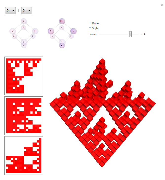
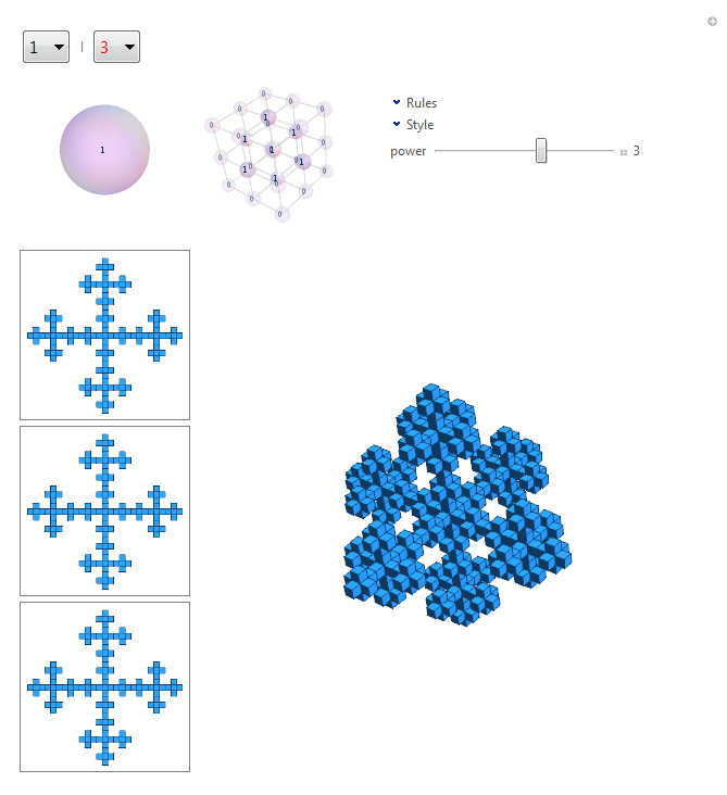
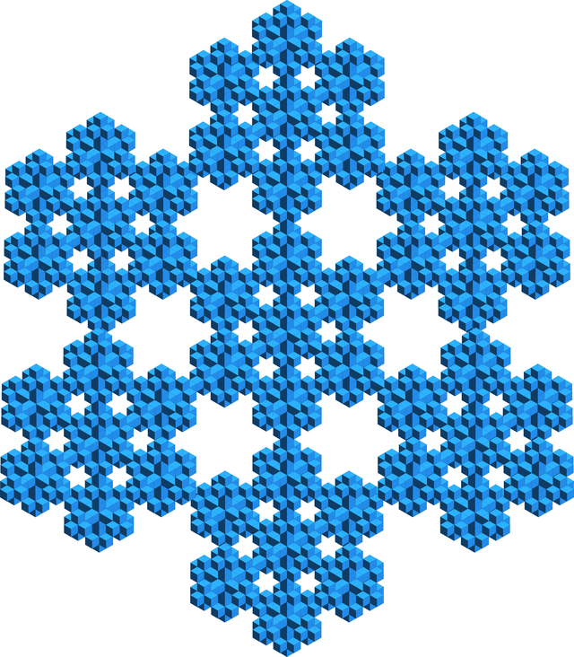
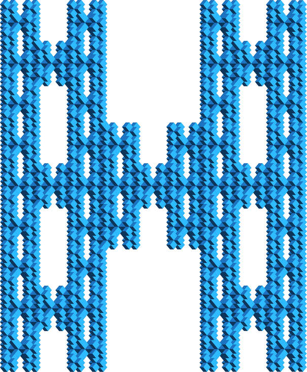
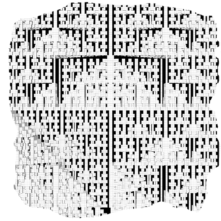
This scheme clearly shows the projective character of these algorithms. Take for example this nifty 3D plus sign made of 3D plus signs, holy mathphobia inducer. It looks like a 2D fractal plus sign when viewed along each axis, but resembles various 2D constructions when viewed from mixed angles.

What's not obvious from these images is that the matrix controls at the top (the pink spheres) and the output figure share the same viewpoint (twirl one, the other two follow). In Mathematica this is as easy as wrapping a couple of things in Dynamic[ ], after which the system takes care of automatically updating things as necessary. It's pretty much the ideal of what event handling should be, at least for these kinds of applications. The underlying engineering for this on Mathematica's part must be very intricate.

And speaking of intricate, this is probably the most complicated Mathematica program I've so far written, in part because I didn't run it through any last-phase refactoring. If you have the courage to fiddle with this program (and I encourage you to have this courage, as the program has a particular issue I couldn't solve), be prepared to suffer dearly for my laziness.

Give me a moment.

OK, it looks like we're in the inversion section. Where did all this 3D stuff come from? Holy cow. HOLY BRAHMAN DATA COW. Oh I think I know which voice it was. Irregardless, since a bunch of 3D things essentially just programmed themselves into existence while I wasn't looking, this means we can do 3D INVERSIONS!!!! Chaos game.

draw[vertices_, numPts_] :=
  Graphics3D[{PointSize[0], Opacity[.1],
    Point[FoldList[(#1 + #2)/2 &, .5 First[vertices],
      RandomChoice[N@vertices, numPts]]]},
   Boxed -> False];

invert[p_] := p/Norm[p]^2;

vertices = PolyhedronData[{"Pyramid", 3}, "VertexCoordinates"];
vertices = Normalize /@ (# - Mean[vertices] &) /@ vertices;

Show[
 draw[vertices, 20000],
 draw[vertices, 100000] /. Point[pts_] :> Point[invert /@ pts]]

This. Four-headed tri-jawed infinity-mouthed Pac-man langolier. If the world ever decides to give me a nightmare, I hope it picks one of these adorable things to chase me through the dark recesses of my deranged mind. Geometric.

draw[shape_, n_] := Module[{next},
   (*scale by 1/2 toward each vertex, in turn*)
   next[prev_] := Scale[prev, 1/2, #] & /@ shape[[1]];

   Graphics3D[{EdgeForm[Opacity[.15]],
     Nest[next, N@shape, n]},
    Lighting -> "Neutral", Boxed -> False]];

invert[p_] := p/Norm[p]^2;

shape = PolyhedronData[{"Pyramid", 3}, "Faces"];
shape[[1]] = Normalize /@ (# - Mean[shape[[1]]] &) /@ shape[[1]];

Show[
 draw[shape, 3],
 (draw[shape, 4] // Normal) /.
  Polygon[pts_, __] :> Polygon[invert /@ pts]]

The ostensive architectonics, quite awesome. c.f. Dyson sphere. The code however is simple. Cobra.

draw[shape_, n_] := Module[{next},
   (*scale by 1/2 toward each vertex, in turn*)
   next[prev_] := Scale[prev, 1/2, #] & /@ shape[[1]];

   Graphics3D[{EdgeForm[Opacity[.15]],
     Opacity[.75], Black, Nest[next, N@shape, n]},
    Lighting -> "Neutral", Boxed -> False]];

transform[1][p_] := p^3/Norm[p]^2;
transform[2][p_] := (Reverse[p].p) p/Norm[p]^2;
transform[3][p_] := (Reverse[p].Cross[{0, 0, 1}, p]) p/Norm[p]^2;

shape = PolyhedronData[{"Pyramid", 3}, "Faces"];

(draw[shape, 4] // Normal) /.
  Polygon[pts_, __] :> Polygon[transform[1] /@ pts]

And fishie! Logarithmic.

game = Compile[{{vertices, _Real, 2}, {w, _Real}, {numpoints, _Integer}},
   Module[{diff},
    FoldList[(diff = #2 - #1;
       Clip[(#1 + #2) Log[Sqrt[diff.diff] + w]]) &,
     {0, 0, 0}, RandomChoice[vertices, numpoints]]]];

invert[p_ /; Norm[p] < .25] := 4 Normalize[p];
invert[p_] := p/Norm[p]^2;

vertices = PolyhedronData[{"Pyramid", 3}, "VertexCoordinates"];
(*vertices=Normalize/@(#-Mean[vertices]&)/@vertices;*)

Graphics3D[{PointSize[0], Opacity[.2],
  Point[invert /@ game[vertices, .01, 400000]]},
 Boxed -> False]

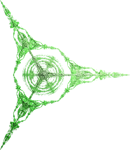
"Chaos game with logarithmic distance function" is a bit long. We need to give this specific kind of fractal a name. What about "Charlie render"? So I'd be like "here we have an inverted Charlie render at w factor .01" and people would nod comprehendingly while reading that, as if there were an established literature on Charlie renders.

You might object that the contours of this nomenclature don't quite align with the striking yet oft- hauntingly quiescent leylines of its intended referents, but you would be wrong — the matching is nigh onomatopoeial per my linguistic auteurity. Incidentally, you should see what my writing looks like when I really cut loose. Rejoice asplendent my sparing you that paragon 'cross the rubicon, padawan.

Since the originals have a lot of points close to 0, their inverses have a lot of points at very large distances. In this case I've decided to clamp the maximum distance of points to a short range (essentially putting them on a leash, like those ball & chain dogs in Mario Bros. 3). It's another way of dealing with infinities. I like this approach because it preserves the radial texture of the figure, snowglobe-like. Taking this to its conclusion, we normalize all points to the same distance:

game = Compile[{{vertices, _Real, 2}, {w, _Real}, {numpoints, _Integer}},
   Module[{diff},
    FoldList[(diff = #2 - #1;
       Clip[(#1 + #2) Log[Sqrt[diff.diff] + w]]) &,
     {0, 0, 0}, RandomChoice[vertices, numpoints]]]];

vertices = PolyhedronData[{"Pyramid", 3}, "VertexCoordinates"];
(*vertices=Normalize/@(#-Mean[vertices]&)/@vertices;*)

Module[{pts},
 pts = game[vertices, .01, 400000];

 Graphics3D[{
   {Glow[White], Sphere[{0, 0, 0}, .99999]}, PointSize[0], Opacity[.5],
   Point[Normalize /@ pts,
    VertexColors -> (ColorData["AvocadoColors"] /@ Norm /@ pts)]},
  ViewPoint -> {Sqrt[3], -Sqrt[8], 1}, Boxed -> False]]

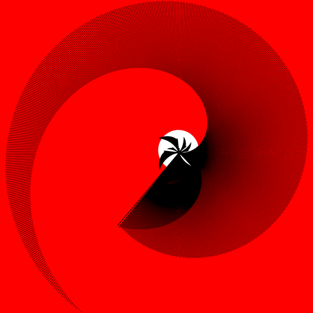
These two are the same, except the first one has an opaque sphere in the interior so that you can't see points beyond the horizon. The extra points in the second one are on the other side of the globe. These points are colored according to their original distance. And the unnormalized figure.

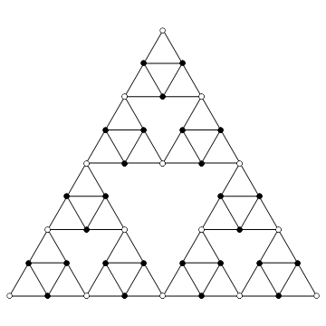
Questions

How many points does the Sierpinski triangle have, besides infinity? Say at a given iteration?

axiom = Polygon[{{0, 0}, {1, Sqrt[3]}/2, {1, 0}}];

next[prev_] := prev /. Polygon[{p1_, p2_, p3_}] :> {
     Polygon[{p1, (p1 + p2)/2, (p1 + p3)/2}],
     Polygon[{p2, (p2 + p3)/2, (p1 + p2)/2}],
     Polygon[{p3, (p1 + p3)/2, (p2 + p3)/2}]};

draw[n_] := Module[{g},
   g = Graphics[{
      White, EdgeForm[Black],
      Nest[next, axiom, n]}];

   Show[
    (g // next) /. p : Polygon[pts_] :>
      {p, Black, Disk[#, (1/2)^(n + 5)] & /@ pts},
    g /. Polygon[pts_] :>
      {EdgeForm[None], Disk[#, (1/2)^(n + 5.075)] & /@ pts}]];

FindSequenceFunction[
  Length@DeleteDuplicates@
      Cases[draw[#], Disk[p_, ___] :> p, Infinity] & /@ Range[6]
  ][n]

If my web search kune do hasn't failed me, this would make most of our algorithms "geometric space and therefore time" (GSATT) algorithms. Actually I just made that up, I don't know what they're called. It's not really relevant for us since the geometricness also means we get a large number of points with few iterations.

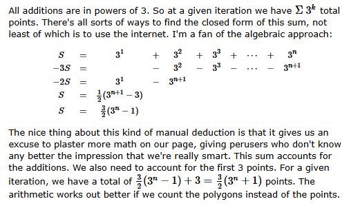
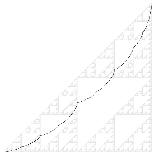
What does the "integration" of the Sierpinski triangle look like? There's various ways to interpret this in 2D, but I'm curious about how the number of points of the triangle increases along a straight line, as if the triangle were a single-variable function:

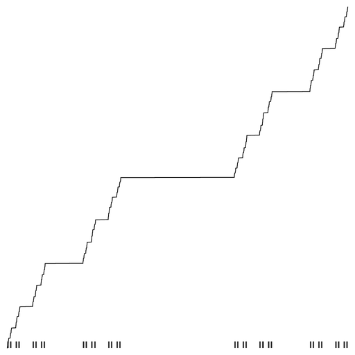
next[prev_] := prev /. Interval[{a_, b_}] :> {
     Interval[{a, a + (b - a)/3}],
     Interval[{a + 2 (b - a)/3, b}]};

cantor[n_] := IntervalUnion @@ Flatten@
    Nest[next, N@Interval[{0, 1}], n];

rectangles[n_, h_: .02, scale_: 1] :=
  Nest[next, Interval[{0, 1}], n] /. Interval[{a_, b_}] :>
    Rectangle[{a, -h (n + 10 h) scale}, {b, -h (n + 1) scale}];

(*this "integration" depends on the "curve" being "uniformly sampled"*)
int[pts_] := MapIndexed[{##} /.
     {{x_, y_}, {i_}} :> {x, i} &, SortBy[pts, First]];

set = cantor[16];(*this is 2^16 intervals*)
{null, {pts}} = Reap[Do[
   If[IntervalMemberQ[set, a], Sow[{a, 0}]],
   {a, 0., 1., 1/1000000}]];

Graphics[rectangles /@ Range[6]]

Show[Graphics[rectangles[6] /.
   Rectangle[{x1_, y1_}, {x2_, y2_}] :> Rectangle[{x1, 0}, {x2, .02}]],
 ListLinePlot[{#1, #2/Length[pts]} & @@@ int[pts],
  PlotStyle -> Black]]

axiom = Polygon[{{0, 0}, {1, 0}, {1, 1}}];

next[prev_] := prev /. Polygon[{p1_, p2_, p3_}] :> {
     Polygon[{p1, (p1 + p2)/2, (p1 + p3)/2}],
     Polygon[{p2, (p2 + p3)/2, (p1 + p2)/2}],
     Polygon[{p3, (p1 + p3)/2, (p2 + p3)/2}]};

points[n_] := DeleteDuplicates[Flatten[
    Nest[next, N@axiom, n] /. Polygon -> Sequence, n]];

(*this "integration" depends on the "curve" being "uniformly sampled"*)
int[pts_] := MapIndexed[{##} /.
     {{x_, y_}, {i_}} :> {x, i} &, SortBy[pts, First]];

pts = points[10];

Show[
 Graphics[{Opacity[.1], PointSize[0], Black, Point[pts]}],
 ListLinePlot[{#1, #2/Length[pts]} & @@@ int[pts], PlotStyle -> Black]]

Hmm. I was hoping it would look something like the so-called Devil's Stairscase, which is the same thing for the Cantor set. You can just feel the Staircase's ragged darkness filling you with joy. But this, this looks like the underside of a fluffy cloud. I think I will call it Lumpy Space Satan's Hairline. Not as dark and morally grimy a name as I was hoping to coin, but not bad either.

My original reason for inverting the Sierpinksi triangle was to see how it might magnify the inner texture. I.e. turning the triangle inside out to make the inside more visible. "You could have explained that in the actual inversion section" you say. Indeed, but let's not hark on couldas and shouldas. The point is there is an intuition behind these things, and we can ask other questions in the same spirit. For example, what if we extend the 2D Sierpinski triangle into 3D, with each point a different z coordinate (depth) depending on its distance from the center of the triangle?

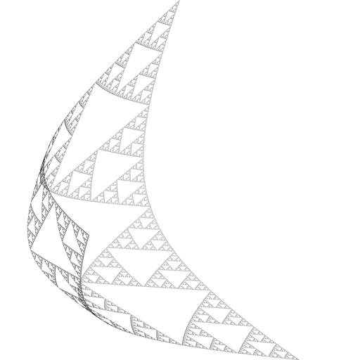
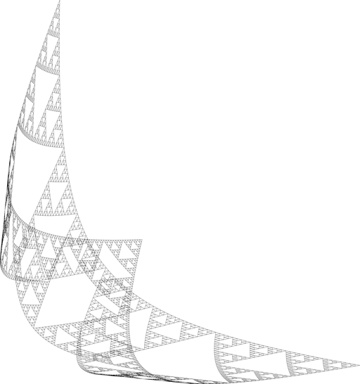
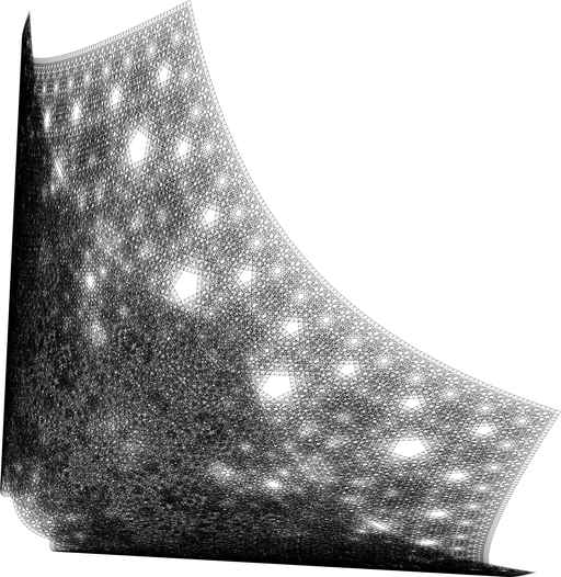
draw[v_, n_] := Module[{ring, figure},
   ring[c_, r_, depth_] := Module[{ps},
     ps = c + r {Cos[#], Sin[#]} & /@ (2 Pi Range[v]/v);

     If[depth == 0, Polygon[ps],
      ring[(c + #)/2, r/2, depth - 1] & /@ ps]];

   figure = ring[0., 1., n] /. Polygon[pts_] :>
      Polygon[{#1, #2, Norm[{#1, #2}]} & @@@ pts];

   (*figure=ring[0.,1.,n]/.Polygon[pts_]:>
   Polygon[Normalize[#]~Append~Norm[#]&/@pts];*)

   Graphics3D[{Transparent,
     EdgeForm[{Opacity[.5], Black}], figure}]];

draw[3, 5]

We get what we expect, a boomerang-looking thing. And look at this lovely demonic-looking Moire pattern, surely the universe's recompense for that fluffy cloud nonsense above. We can also normalize the points so that all we see is the radial detail. That produces a coronet-looking thing, which can be unrolled:

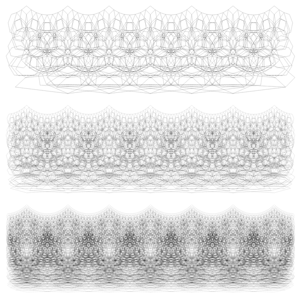
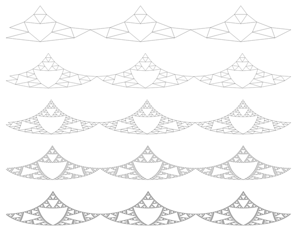
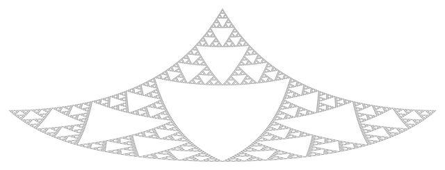
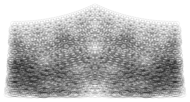
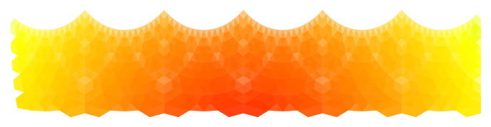
draw[v_, n_, s_: 2, cutoff_: 0, width_: 1] := Module[{ring, figure},
   ring[c_, r_, depth_] := Module[{ps},
     ps = c + r {Cos[#], Sin[#]} & /@ (2 Pi Range[v]/v);

     If[depth == 0, Polygon[ps],
      ring[(c + #)/2, r/2, depth - 1] & /@ ps]];

   figure = ring[0., 1., n] /. Polygon[pts_] :>
      Polygon[{ArcTan @@ (# /. {0., 0.} -> {1., 0.}), s Norm[#]} & /@ pts];
   figure = Flatten[figure];

   figure = Cases[figure, Polygon[pts_] /;
      Mean[Norm /@ Differences[pts]] < .5
       (*&&MemberQ[First/@pts,a_/;-width Pi/v<a<width Pi/v]*)
       && MemberQ[Last /@ pts, y_ /; y > cutoff s]];

   Graphics[{Opacity[.5],
     EdgeForm[{Opacity[.13], JoinForm["Round"]}],
     figure}, ImageSize -> Large]];

draw[6, 4, 2, .4] /. Polygon[pts_] :>
  {Opacity[.5], EdgeForm[{Opacity[.01], LightGray}],
   Hue[.05 Norm[Mean[pts]]], Polygon[pts]}

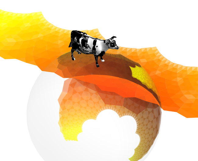
What does a radial histogram of the Sierpinski triangle look like?

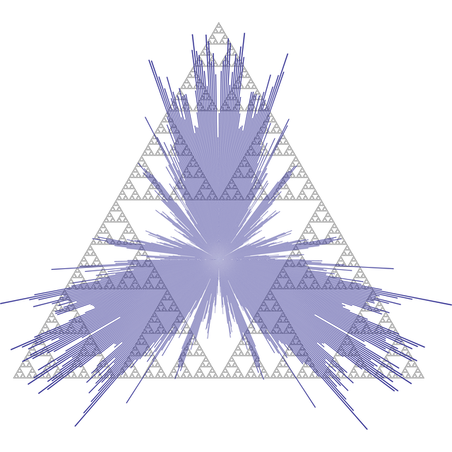
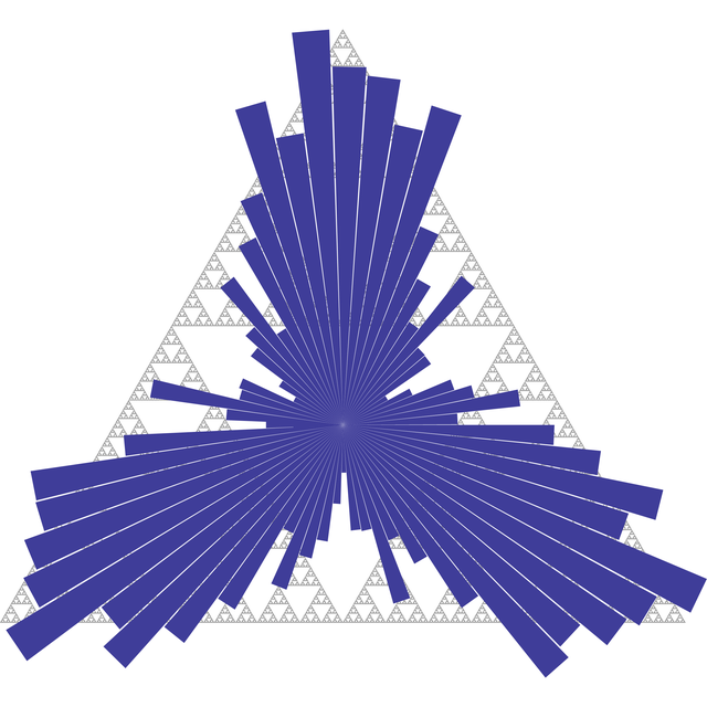
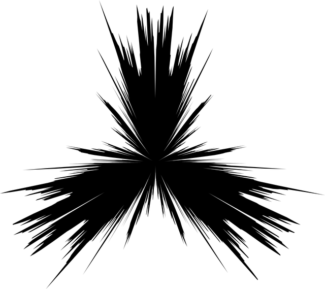
axiom = Polygon[{Cos[#], Sin[#]} & /@ (Pi/2 + 2 Pi Range[3]/3)];

next[prev_] := prev /. Polygon[{p1_, p2_, p3_}] :> {
     Polygon[{p1, (p1 + p2)/2, (p1 + p3)/2}],
     Polygon[{p2, (p2 + p3)/2, (p1 + p2)/2}],
     Polygon[{p3, (p1 + p3)/2, (p2 + p3)/2}]};

points[n_] := DeleteDuplicates[Flatten[
    Nest[next, N@axiom, n] /. Polygon -> Sequence, n]];

pts = points[8];
stats = Transpose@MapAt[Partition[#, 2, 1] &, #, 1] &@
   HistogramList[ArcTan @@@ pts, "Knuth"];

max = Max[Last /@ stats];
polys = Polygon[#2/max {{0, 0},
       {Cos[#1[[1]] + .005], Sin[#1[[1]] + .005]},
       {Cos[#1[[2]]], Sin[#1[[2]]]}}] & @@@ stats;
(*poly=Polygon[#2/max{Cos[#1[[1]]],Sin[#1[[1]]]}&@@@stats];*)

Graphics[{
  {PointSize[0], Opacity[.1], Point[pts]},
  {ColorData[1][401], polys}}]

What happens if we run the Game of Life on the Sierpinski triangle?

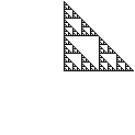
sier[n_] := Mod[Array[Binomial, {n, n}, 0], 2];

s = ArrayPad[sier[2^9], 2^5];
(*s=sier[2^9]+Transpose[sier[2^9]]/. 2->1;*)
i = 0;

PrintTemporary[Dynamic[i]];
PrintTemporary[Dynamic[Image[s]]];

With[{lifeSpec = {224, {2, {{2, 2, 2}, {2, 1, 2}, {2, 2, 2}}}, {1, 1}}},
  While[i++ < Infinity,
   s = CellularAutomaton[lifeSpec, s]]];

i
Image[s]

Basically nothing. The triangle does this and that, shoots a couple gliders, settles. Larger versions do more or less the same thing but take longer to settle. Not very interesting, but it raises the idea of using fractals as starting configurations. However, on the internet I found that lines produce Sierpinski triangles:

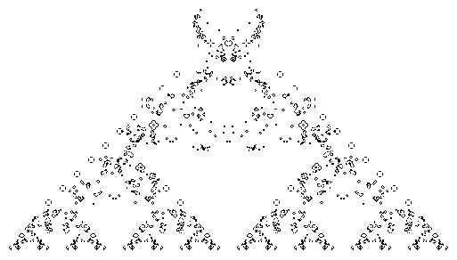
Export["c:/users/zrp/desktop/line.bmp",
 Image[{ConstantArray[0, 2^13]}]]

With[{lifeSpec = {224, {2, {{2, 2, 2}, {2, 1, 2}, {2, 2, 2}}}, {1, 1}}},
  frames = CellularAutomaton[lifeSpec,
    {{ConstantArray[1, 2^8(*-14*)]}, 0}, 130]];

Export["c:/users/zrp/desktop/zrp.gif",
 ColorNegate /@ Image /@ frames, "DisplayDurations" -> .17]

With[{lifeSpec = {224, {2, {{2, 2, 2}, {2, 1, 2}, {2, 2, 2}}}, {1, 1}}},
  frames = CellularAutomaton[lifeSpec,
    Boole@Array[#1 == 2^7 &, 2^8 {1, 1}], 2^7]];

Export["c:/users/zrp/desktop/zrp.gif",
 ColorNegate /@ Image /@ frames, "DisplayDurations" -> .17]

I didn't even have to add the horns. This is one end of a line after some iterations. The pattern continues propagating forever and ever as long as there is line left and becomes more distinguished at larger scales. It appears to be driven entirely by the line itself. Consider the evolution of a line that is infinitely long, something you can actually witness in the Game of Life by connecting the edges of the board.

As the finite line splits, it leaves debris due to the circumstances of the ends. The pattern you end up with is a trace of the line's subdivisions. It's because the line splits cleanly and does so in a Sierpinski recursion that you end up with clear Sierpinski triangles at larger scales.

If you want to play with large Game of Life constructions, the easiest way is to export them as images and open them in a dedicated Game of Life program, as those can run the game at very high speeds.

What does a random walk on the Sierpinski graph look like?

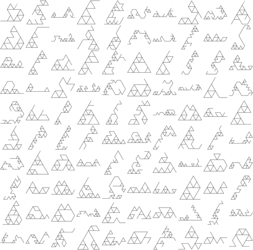
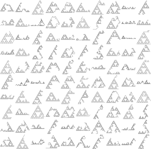
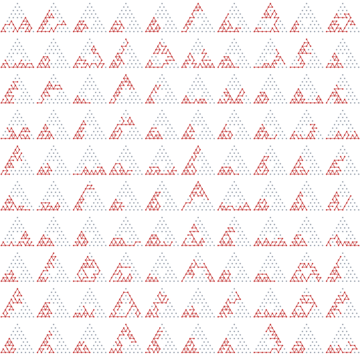
axiom = Polygon[{{0, 0}, {1, Sqrt[3]}/2, {1, 0}}];

next[prev_] := prev /. Polygon[{p1_, p2_, p3_}] :> {
     Polygon[{p1, (p1 + p2)/2, (p1 + p3)/2}],
     Polygon[{p2, (p2 + p3)/2, (p1 + p2)/2}],
     Polygon[{p3, (p1 + p3)/2, (p2 + p3)/2}]};

draw[n_] := Module[{edges},
   edges = Flatten@Nest[next, N@axiom, n] /. Polygon[pts_] :>
      Sequence @@ UndirectedEdge @@@ Partition[pts, 2, 1, 1];

   Graph[edges, VertexCoordinates -> VertexList[Graph[edges]],
    VertexSize -> .25]];

graphWalkPath[g_Graph, steps_: 15] := Module[{neighbors},
   neighbors[vertex_] := (neighbors[vertex] =
      Complement[VertexList[NeighborhoodGraph[g, vertex]], {vertex}]);

   NestList[RandomChoice[neighbors[#]] &, First[VertexList[g]], steps]];

SetAttributes[UndirectedEdge, Orderless];
graphWalk[args__] := Graph[DeleteDuplicates[
    UndirectedEdge @@@ Partition[graphWalkPath[args], 2, 1]]];

g = draw[3];
Grid[Partition[#, 10]] &@Table[
  Graphics[{Opacity[.8], JoinForm["Round"], Line[graphWalkPath[g, 50]]},
   ImageSize -> 50 {1, 1}], {100}]

Grid[Partition[#, 10]] &@Table[
  HighlightGraph[g, graphWalk[g, 50],
   ImageSize -> 50 {1, 1}], {100}]

About what you would expect. I'll leave the stats to those whose laziness is bounded from above, instead of below. What does a "circle" look like on the Sierpinski graph?

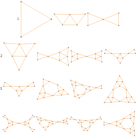
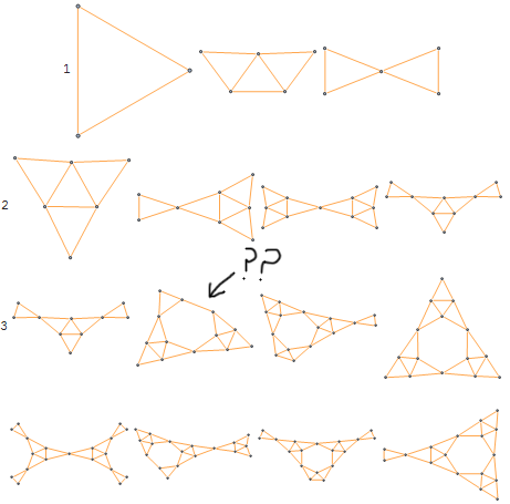
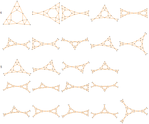
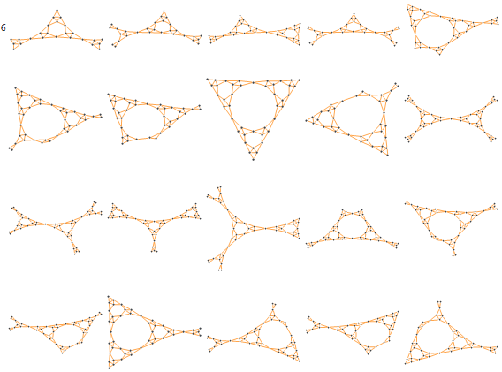
axiom = Polygon[{{0, 0}, {1, Sqrt[3]}/2, {1, 0}}];

next[prev_] := prev /. Polygon[{p1_, p2_, p3_}] :> {
     Polygon[{p1, (p1 + p2)/2, (p1 + p3)/2}],
     Polygon[{p2, (p2 + p3)/2, (p1 + p2)/2}],
     Polygon[{p3, (p1 + p3)/2, (p2 + p3)/2}]};

draw[n_] := Module[{edges},
   edges = Flatten@Nest[next, N@axiom, n] /. Polygon[pts_] :>
      Sequence @@ UndirectedEdge @@@ Partition[pts, 2, 1, 1];

   Graph[edges, VertexCoordinates -> VertexList[Graph[edges]],
    VertexSize -> .25]];

style = Sequence[EdgeStyle -> Orange];
circles[g_Graph, r_: 1] := (circles[g, r] =
    Module[{vs = VertexList[g]},
     DeleteDuplicates[
      NeighborhoodGraph[g, #, r, style] & /@ vs,
      IsomorphicGraphQ]]);

Pane[#, 600] &@Column[
  Row[Prepend[
      circles[draw[5], #],
      Style[#, Lighter[Black, 1/6]]], " "] & /@ Range[1, 3],
  Alignment -> Center, Spacings -> 1]

This brings to light a more important question: What the hell is this? It's like the ugly duckling of radius 3 Sierpinski subgraphs. Just look at it. LOL. But OK, I mightn't myself be the most handsomest chap on the block, and graphs are people too after all.

There's a good chance that subgraph is hideous because it contains one of the 3 end vertices of the graph as a whole, though I'm too lazy to check this. Those vertices are in part pathological because they have degree 2, whereas all the other vertices have degree 4. But really I think the Sierpinski graph itself is contrived. At least, the finite version seems contrived to me.

Perhaps because the Sierpinski pattern might actually be a grid, in the sense that the empty space is an integral part of its characterization a la our infinite quadrilateral descent construction. If we base a graph on the pattern produced by the mod 2 binomial, we get this graph:

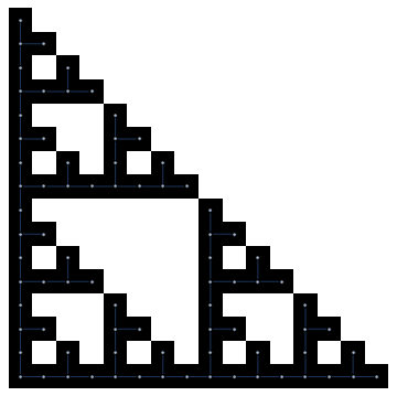
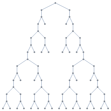
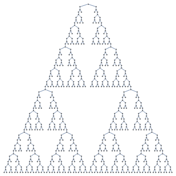
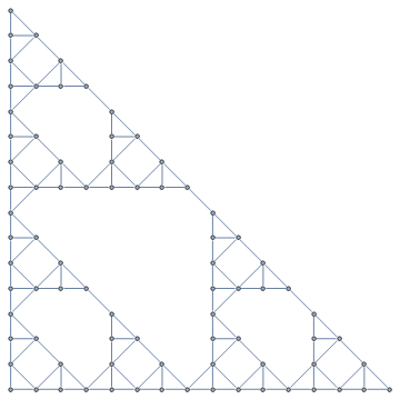
locs[n_] := RotationTransform[-Pi/2] /@
   Position[Mod[Array[Binomial, {n, n}, 0], 2], 1];

draw[n_, grid_: True] :=
  Module[{edges, subsets = Subsets[locs[n], {2}]},
   edges = UndirectedEdge @@@
     Pick[subsets,
      ManhattanDistance(*;ChessboardDistance*)@@@ subsets, 1];

   Graph[edges, VertexCoordinates -> If[grid,
      {.5, .5} + # & /@ VertexList[Graph[edges]]]]];

Show[
 Graphics[Rectangle /@ locs[2^4]],
 draw[2^4]]

Which looks like this in a tiered layout. Maybe the "real" Sierpinski graph is a binary tree of this sort, and it's only connected on all sides in the infinite case. And maybe right now I'm making mathematicians bash their heads against walls, which would be awesome.

The binomial mod 2 construction was one of the approaches that went AWOL during our 3Dification blitz. Does it have a 3 dimensional version? Yes, the multinomial mod 2. The code is almost as pretty as it is for the 2D version:

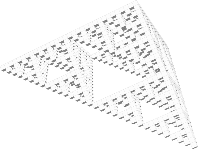
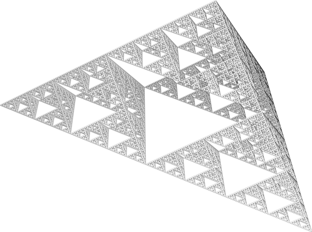
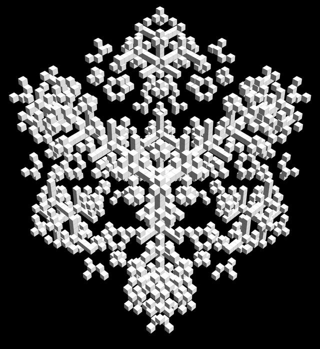
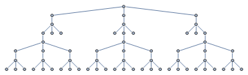
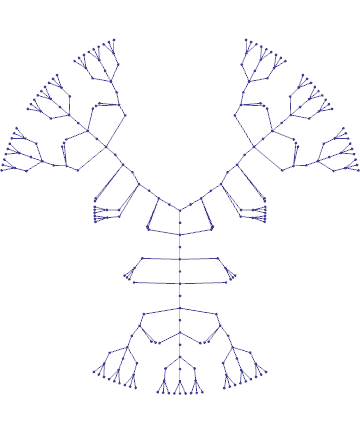
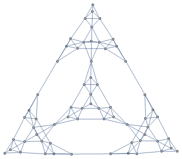
array[n_] := Mod[Array[Multinomial, n {1, 1, 1}, 0], 2];

draw[n_] := Graphics3D[Cuboid /@ Position[array[n], 1],
   Lighting -> "Neutral", Boxed -> False];

array[n_] := Mod[Array[Multinomial, n {1, 1, 1}, 0], 2];

draw[n_] := Module[{edges, subsets},
   subsets = Subsets[Position[array[n], 1], {2}];

   edges = UndirectedEdge @@@
     Pick[subsets,
      ManhattanDistance(*;ChessboardDistance*)@@@ subsets, 1];

   Graph[edges]];

draw[2^3]
GraphPlot3D[draw[2^3], PlotStyle -> ColorData[1][424]]

Poor Boxed, always being set to False. What happens to our chaos game algorithm if we implement some notion of momentum for the active point?

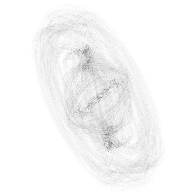
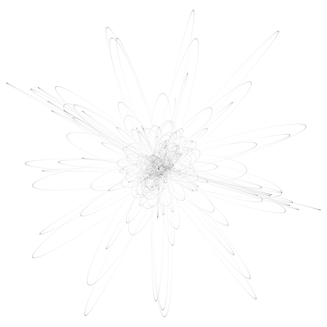
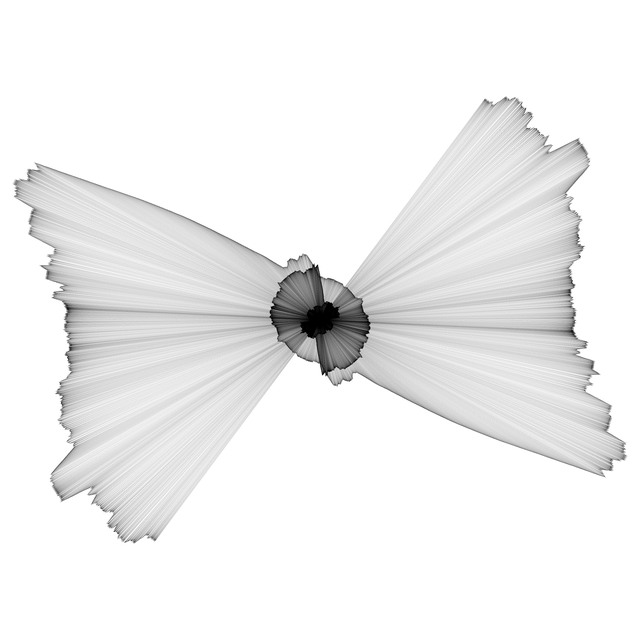
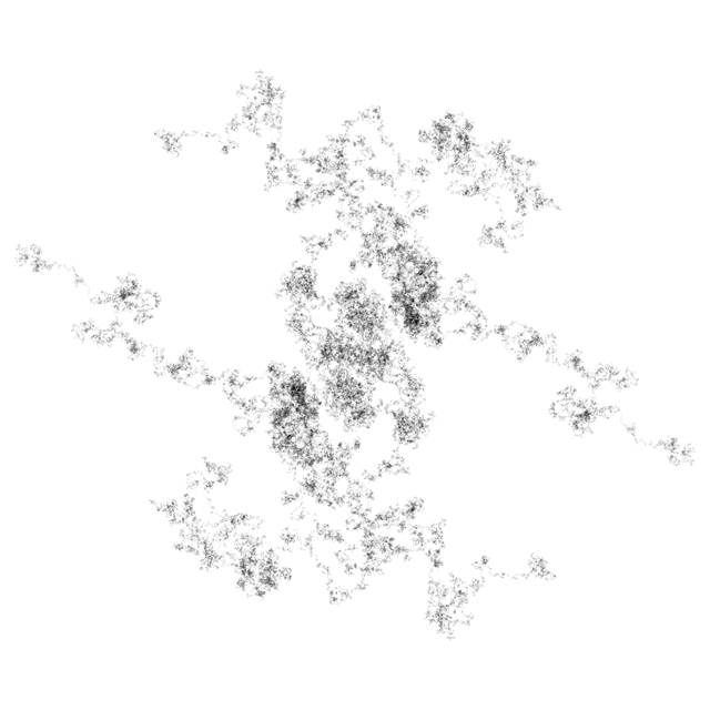
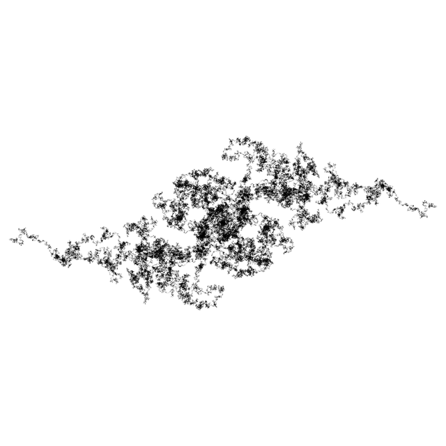
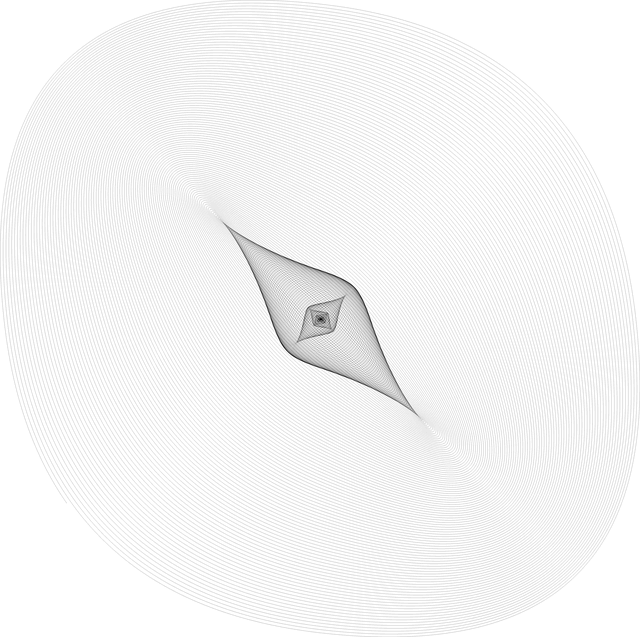
game[v_, numPoints_] := Module[{vertices, update, vl},
   vertices = {Cos[#], Sin[#]} & /@ (2 Pi Range[v]/v);

   update[{pos0_, vl0_}, nextVertex_] := (
     (*vl=vl0+(pos0+nextVertex)/650-pos0;*)
     (*vl = vl0+Normalize[nextVertex - pos0];*)
     vl = vl0 + .0001 (nextVertex - pos0);
     {pos0 + vl, vl});

   First /@ FoldList[update, N@{{0, 0}, {0, 0}},
     RandomChoice[N@vertices, numPoints]]];

Graphics[{PointSize[0], Opacity[.1],
  Point[game[3, 100000]]}]

game[v_, numPoints_] := Module[{vertices, update, vl},
   vertices = {Cos[#], Sin[#]} & /@ (2 Pi Range[v]/v);

   update[{pos0_, vl0_}, nextVertex_] := (
     vl = vl0 + Clip[(nextVertex - pos0), 20 {-1, 1}];
     {pos0 + vl, vl});

   First /@ FoldList[update, N@{{0, 0}, {0, 0}},
     RandomChoice[N@vertices, numPoints]]];

zrp = ParallelTable[Module[{pts, max, maxx, maxy},
    pts = game[4, n];
    max = Sqrt[2] Max[Abs /@ pts];

    SeedRandom[400, Method -> "ExtendedCA"];
    Rasterize@Graphics[{Opacity[.9], Line[pts]},
      PlotRange -> max, ImageSize -> {150, 150}]],
   {n, 1, 10000, 83}];

Export["c:/users/zrp/desktop/zrp.gif",
 ColorQuantize[#, 4] & /@ Most[zrp]]

I didn't find any interesting formulas, but still I managed to get a variety of figures by fiddling with numbers. Probably I would have to use math to find something more interesting.

The figures have precise symmetries (180 degree rotation), apparently because the particle eventually overshoots far enough that the randomness becomes a small jitter component (because the vertices of the game become very distant), so it accumulates a near-linear velocity/path on its way back. I'm not sure about this explanation though.

Even the ones that look like random walks are symmetric. They aren't standard random walks, rather the particle is overshooting back and forth. This raises the idea of symmetrizing random walks:

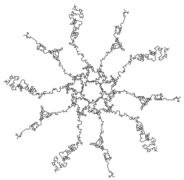
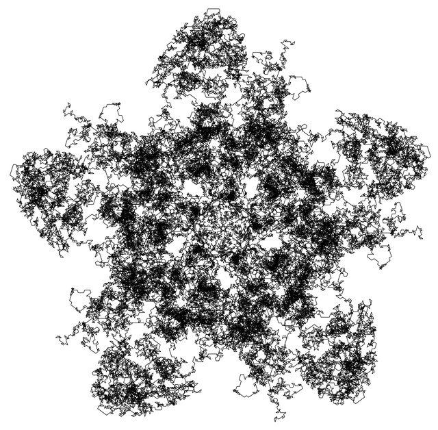
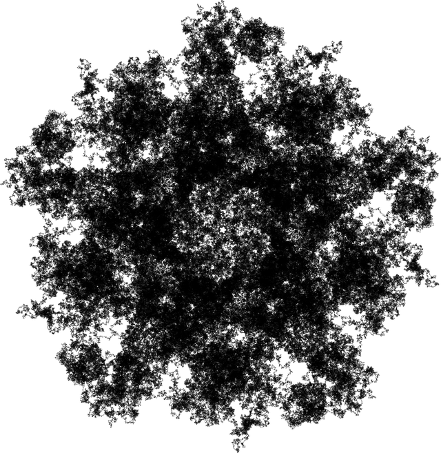
draw[v_, r_, numSteps_: 100] := Module[{directions, walk},
   directions = {Cos[#], Sin[#]} & /@ (2. Pi Range[v]/v);

   walk = Accumulate[RandomChoice[directions, numSteps + 1]];
   Graphics[Rotate[Line[walk], #] & /@ (2. Pi Range[r]/r)]];

Awesome possum. What do you see here? When fiddling with momentum I found a simple variation on the logarithmic distance function:

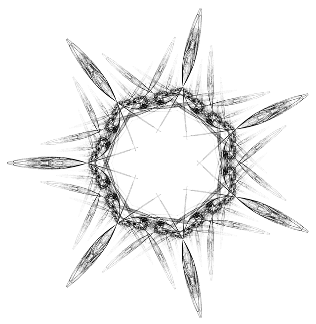
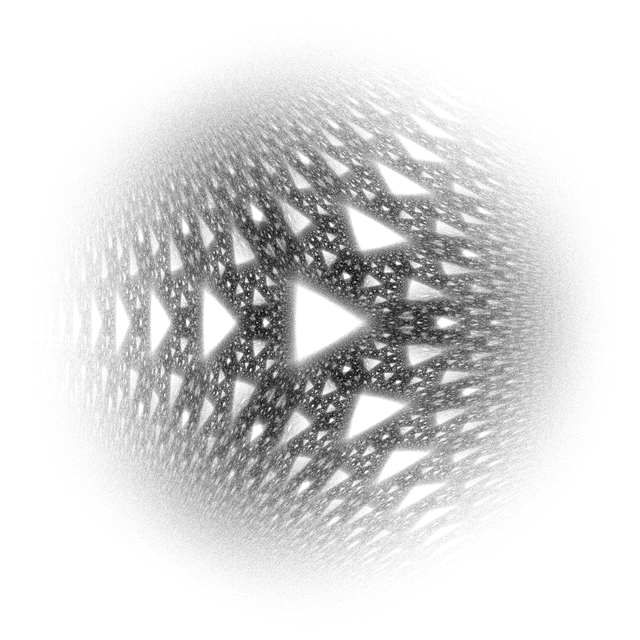
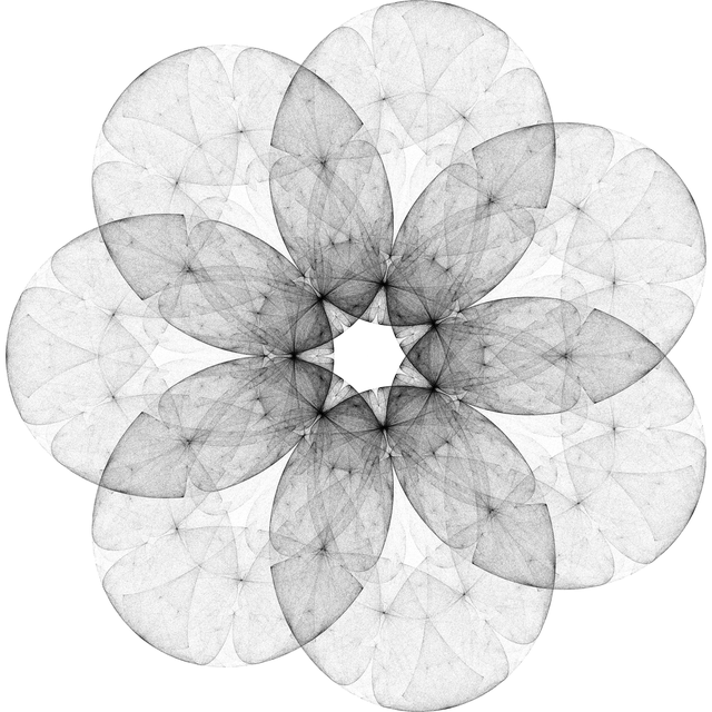
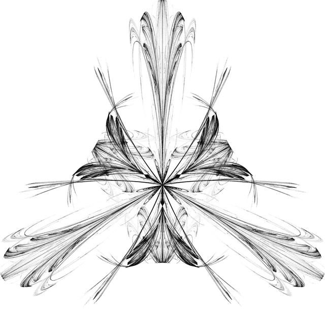
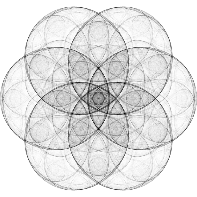
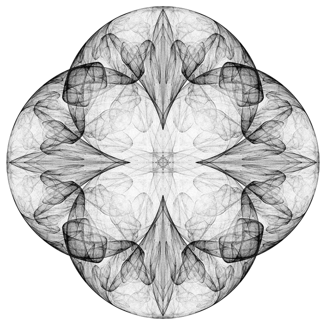
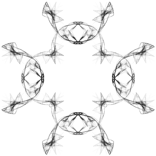
Module[{gameC},
  gameC = Compile[{{spec, _Real, 1}, {numPoints, _Integer, 0}},
    Module[{vertices, diff, v, w, s, b, r, p, z, c},
     {v, w, s, b, r, p, z, c} = spec;
     vertices = {Cos[#], Sin[#]} & /@ (2 Pi Range[v]/v);

     FoldList[(
        diff = #2 - #1;
        p #1 + Clip[(#1 + z #2) Log[b, (diff.diff)^(1/r) + w], c {-1, 1}]) &,
      {0, 0}, RandomChoice[s vertices, numPoints]]]];

  game[spec_, numPoints_] :=
   gameC[PadRight[spec, 8, {3, .5, 1, E, 2, 0, 1, 2}], numPoints]
  ];

draw[spec_, numPoints_: 100000, rot_: 0, style___] := Graphics[{
    PointSize[0], Opacity[.1], style,
    Rotate[Point[game[spec, numPoints]], rot]}];

draw[{5, .8}]

(*{vertex count, w factor, scale, base, root, prefix, polarity, clip range}*)
(*Show[draw[{3, .12, .3, 3.9, .9, 1, -.5 E, 1}, 2000000, -Pi/6],
   ImageSize -> 2 1280] // Rasterize // ImageResize[#, Scaled[1/4]] &*)

Or something of a generalization. I blindly parameterized several parts of the formula. Some of the parameters are sensitive, but in any case it's easy to find spiffy images. The hard part is deciding which of them to put here. 3D version:

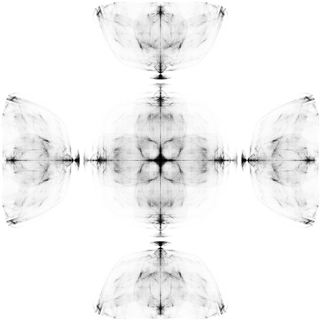
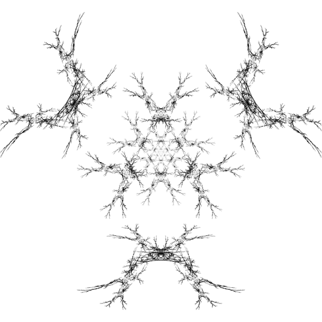
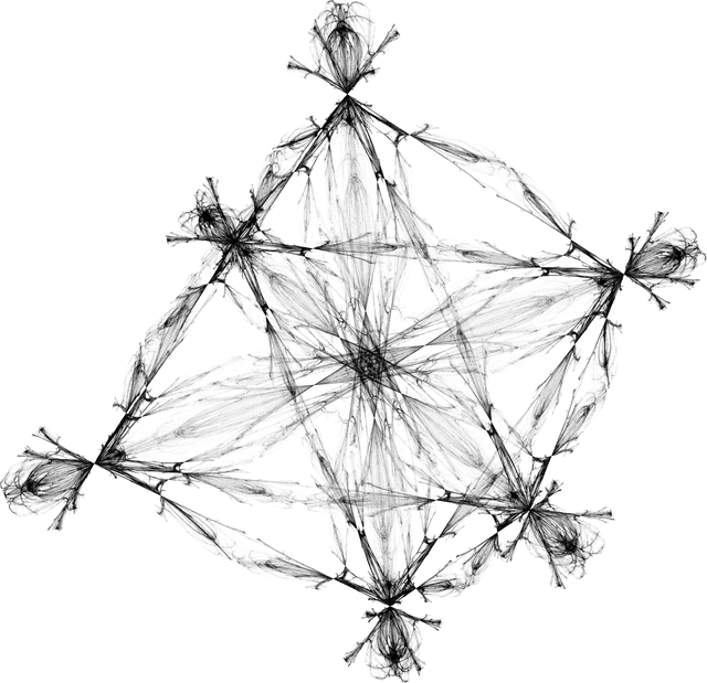
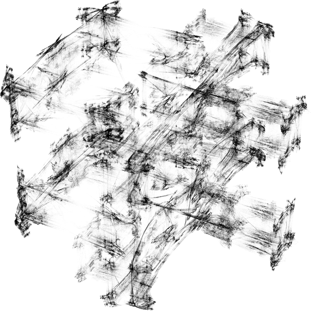
Module[{gameC},
  gameC =
   Compile[{{vertices, _Real, 2}, {spec, _Real, 1}, {numPoints, _Integer, 0}},
    Module[{diff, w, r, s, b, p, z, c},
     {w, s, b, r, p, z, c} = spec;

     FoldList[(
        diff = #2 - #1;
        p #1 + Clip[(#1 + z #2) Log[b, (diff.diff)^(1/r) + w], c {-1, 1}]) &,
      Mean[vertices] RandomReal[], RandomChoice[s vertices, numPoints]]]];

  game[vertices_, spec_, numPoints_: 100000] :=
   gameC[vertices, PadRight[spec, 7, {.5, 1, E, 2, 0, 1, 2}], numPoints]
  ];

draw[vertices_, spec_, numPoints_: 100000, options___] :=
  Graphics3D[{PointSize[0], Opacity[.1],
    Point[game[vertices, spec, numPoints]]},
   options, Boxed -> False];

(*{w factor, scale, base, root, prefix, polarity, clip range}*)

vertices = PolyhedronData[{"Dipyramid", 5}, "VertexCoordinates"];
draw[vertices, {.8}, 200000]

(*note.*)
v2D = {Cos[#], Sin[#]} & /@ (2 Pi Range[5]/5);
{Graphics[Point[game[v2D, {.8}]]],
 Graphics3D[Point[game[{##, 0} & @@@ v2D, {.8}]]]}

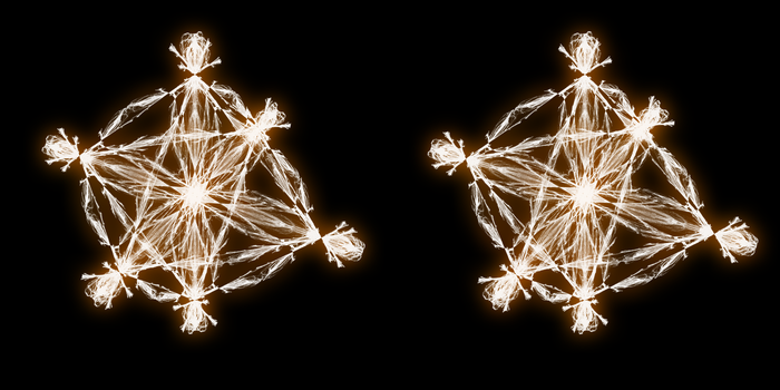
I love how some of these look like sketches. You'd expect to find this as an illustration in a wizard's journal, but it's actually from a Graphics3D pane in my Mathematica notebook. This opportune box, beside being the final confine of a truculent force, is the result of the clipping I use to keep the point from escaping. I set the clipping as a parameter because it can be used to effect.

This clipping restriction isn't always necessary, and it might not be necessary for all points within a given figure, which raises an interesting prospect: What if we try to identify the points that fly off into infinity and those that don't?

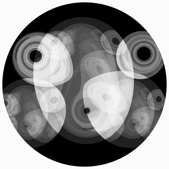
check = Compile[{{c, _Complex, 0}},
   Module[{i = 0, z = 0 I},
    While[
     Abs[z] < Sqrt[2] && i++ < 240,
     z = z^2 + c];
    -i]];

ImageAdjust@Image@
  ParallelTable[check[x + y I],
   {y, -1.1, 1.1, .0035}, {x, -1.55, .6, .0035}]

vertices = (**)5(**) {Cos[#], Sin[#]} & /@ (2 Pi Range[3]/3);

check = Compile[{{x, _Real, 0}, {y, _Real, 0}},
   Module[{i, b, diff, z = {0., 0.}, vertices = vertices},
    Total@Table[
      i = 0; z = {x, y};
      While[z.z < 40 && i++ < 120,
       b = RandomChoice[vertices];
       diff = b - z;
       z = (z + b) Log[Sqrt[diff.diff] + .01]];
      -i,
      {20(*0*)(*number of trials*)}]]];

img = ImageAdjust@Image@
    ParallelTable[check[x, y],
     {y, -6.5, 6.5, .01}, {x, -6.5, 6.5, .01}];

img // Colorize // ImageResize[#, 550] &

Here the white points go off into infinity quickly. The black points don't, or at least they take a lot longer to escape. There are certainly patterns here, but they're much less pronounced and computationally harder to reveal to than they are for the Mandelbrot set, which is the same idea for Julia iterations. But if you spin a few knobs you can find interesting figures irregardless. The different colors/shades are different escape speeds. It may not be immediately apparent, but these are fractals also.

A lot of fractals have scaled/skewed characteristics, including the Mandelbrot set. I wonder if there's a non-trivial chaos game that can create the Mandelbrot set. Since we're skittering around complex numbers, is there an interesting complex-valued version of the logarithmic chaos game?

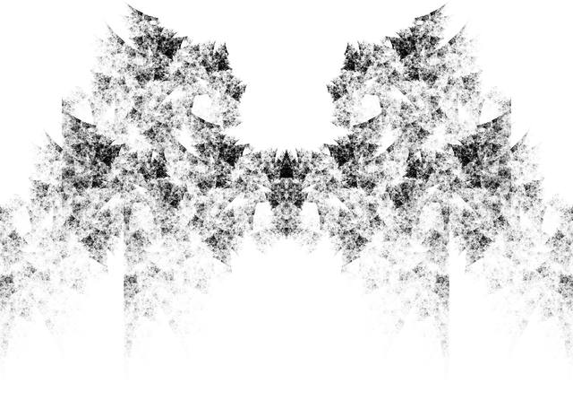
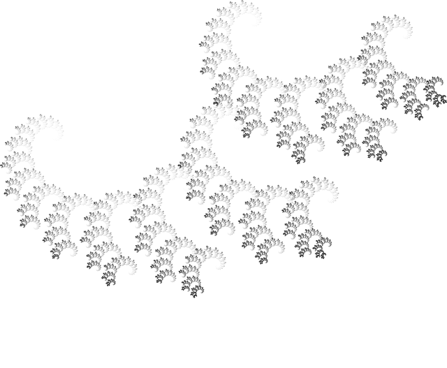
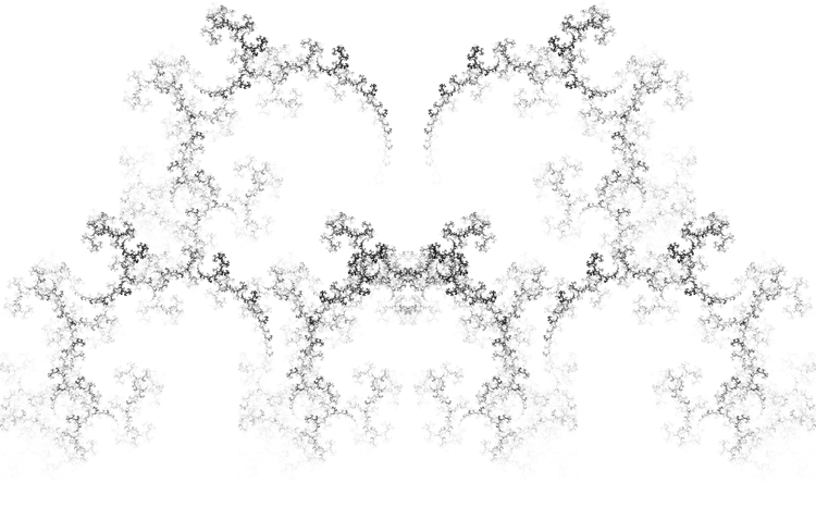
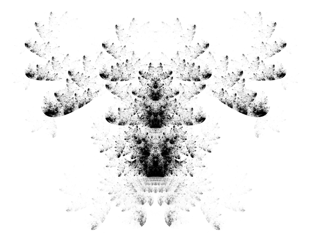
game = Compile[{{v, _Integer, 0}, {numPoints, _Integer, 0}},
   Module[{vertices},
    vertices =(*1.5*)E^(I 2 Pi Range[v]/v);

    FoldList[(*(Log[#1]+#2)/2&*)
     (#1 + (#1 + #2) Log[Sqrt[#2 - #1] + .7])/2.1 &, .1,
     RandomChoice[N@vertices, numPoints]]]];

Graphics[{Opacity[.1], PointSize[0],
  Point[{Im[#], Re[#]} & /@ game[2, 400000]]}]

I don't know. Strictly speaking there wouldn't be a difference, but if you put on a blindfold and chuck logarithms at Mathematica helter-skelter, pretty pictures eventually come out. So I guess the answer is some form of yes. Formally these might still be considered Julia sets.

I've mentioned before that there are a lot of crazy distance functions out there for us to use in our chaos game, and there isn't anything special about the logarithm function. What do plots using other functions look like?

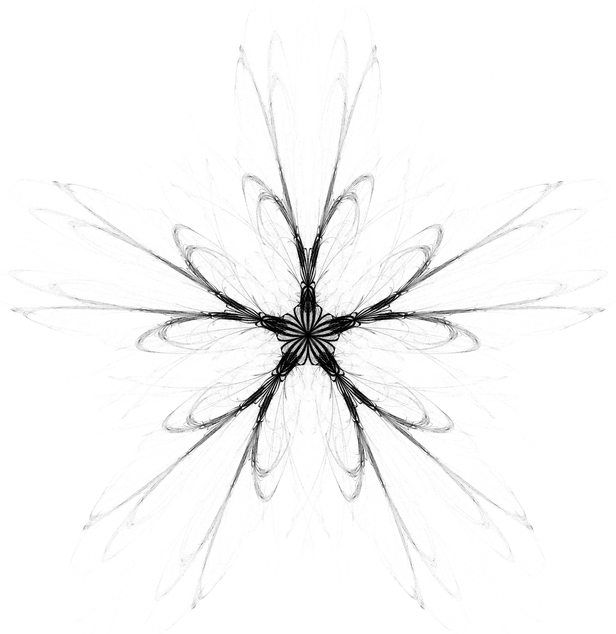
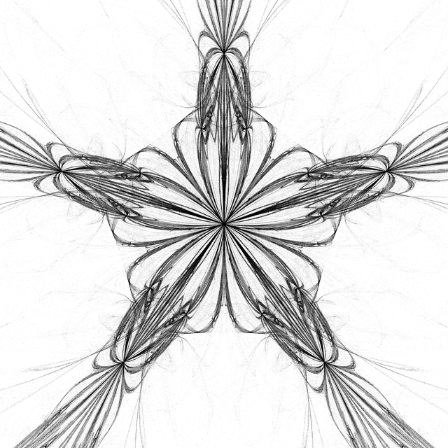
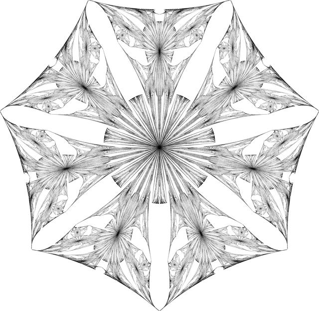
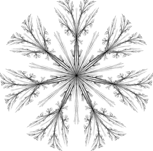
vertices = (**)5(**) {Cos[#], Sin[#]} & /@ (2 Pi Range[3]/3);

check = Compile[{{x, _Real, 0}, {y, _Real, 0}},
   Module[{i, b, diff, z = {0., 0.}, vertices = vertices},
    Total@Table[
      i = 0; z = {x, y};
      While[z.z < 40 && i++ < 120,
       b = RandomChoice[vertices];
       diff = b - z;
       z = (z + b) Sin[Sqrt[diff.diff] + .01]];
      -i,
      {20(*0*)(*number of trials*)}]]];

img = ImageAdjust@Image@
    ParallelTable[check[x, y],
     {y, -6.5, 6.5, .01}, {x, -6.5, 6.5, .01}];

img // Colorize // ImageAdjust // ColorConvert[#, "Grayscale"] & // ImageAdjust //
    ImageResize[#, Scaled[1/2]] & // ImageRotate[#, -Pi/2] & // ColorNegate //
 ImageApply[#^(1/1.3) &, #] &

game[f_, rest__] := rest //
   Compile[{{v, _Integer}, {w, _Real}, {numPoints, _Integer}, {rot, _Real}},
    Module[{diff, tmp, vertices},
     vertices = {Cos[#], Sin[#]} & /@ (rot + 2 Pi Range[v]/v);

     FoldList[(
        diff = #2 - #1;
        tmp = f[Sqrt[diff.diff] + w];
        Clip[(#1 + #2) tmp, 24 {-1, 1}]) &,
      {0, 0}, RandomChoice[vertices, numPoints]]]];

draw[{args__}, rot_: 0, options___] :=
  Graphics[{PointSize[0], Opacity[.25],
    Point[game[args, rot]]}, options];

draw[{Sin, 5, -1.23, 100000}, -Pi/10]
draw[{Cos, 3, Pi/2.675, 100000}, -Pi/6]
draw[{RamanujanTauL, 5, 3.1, 10000}, -Pi/10]

They look just as awesome, of course. Here we have plots using the sine, cosine, and, you guessed it, Ramanujan tau Dirichlet L-function. And this is using the same basic form as the logarithm version, without us even having to put on Loki's mask and get real buckwild. Speaking of masks.

Usually I don't pick favorites, but I like the cosine image (of course sin/cos are just offsets of eachother) because it has an infinite number of folded sheet things that seem to have precise contours. I'll leave the 3Dification as an exercise, but not the how-fast-points-go-to-infinity plot.

The reason it's easy to get all these pictures without trying very hard is that the self-similarity is almost guaranteed by the chaos game algorithm. As we saw earlier, "move toward a point" amounts to the same thing as "make a resized copy of everything toward the perspective of that point."

This is a simplification, but the point is that you essentially get the skeleton of self-similarity for free, or perhaps something a bit more broad. And more abstractly, I think some remarks could be made about the real number system itself.

What does the Sierpinski triangle sound like? One easy interpretation is to consider the L-system construction for the triangle and convert different angles to different frequencies as the turtle makes the triangle:

mp3 midi

mp3 midi

axiom = A;
rules = {A -> {B, R, A, R, B}, B -> {A, L, B, L, A}};
conversions = {A -> forward, B -> forward, L -> left, R -> right};

(*state transformations*)
forward[{z_, theta_}] := {z + E^(I theta), theta};
left[{z_, theta_}] := {z, theta + 2. Pi/6};
right[{z_, theta_}] := {z, theta - 2. Pi/6};

sier[n_] := Module[{program, zs},
   program = Flatten[Nest[# /. rules &, axiom, n]] /. conversions;
   zs = First /@ ComposeList[program, {0, 0}];
   First /@ Split[{Re[#], Im[#]} & /@ zs]];

(*convert angle into the given frequency range*)
freq[min_, max_][angle_] := angle (max - min)/Pi + min;

wave[coords_, dur_: 10, freq_: freq[6, 30]] := Module[{angles, freqs},
   angles = Abs[ArcTan @@@ Differences[coords]];
   freqs = Round /@ freq /@ angles;
   Sound[SoundNote /@ freqs, dur]];

wave[sier[3], 5, freq[8, 15]]

(*overtones zomg*)
Sound[{"NewAge",
  wave[#, {0, 20}] & /@ Table[
    RotationTransform[2 Pi i/4] /@ sier[i], {i, 4}]},
 SoundVolume -> .8]

It sounds totally lame. Not surprising since the L-system construction is simple. There is real power here though. This tonifier operates on coordinate lists of any kind, not just those produced by this particular L-system. And if you do things like layer different iterations on top of each other, you can get nifty chord thingies.

A variation of this would be to determine the waveform directly from the L-system. In a past life I made such a program in C#/WPF. It was around 1200 lines of code. In Mathematica it would be around 30 lines of code, and maybe around 150 lines total with a solid UI around it. It would also be about a million times more powerful/general/flexible. There's a lot of reasons for this, none of which have to do with math.

Luckily for me I don't have to explain. The goddess of finishing projects has finally crawled out of her cave and seen fit to smite her lightning bolt through my ears and across my temporal lobe, for this tune has sated and sedated the voices and quelled their cantankerous echoes. And so ends part 1.