I love how some of these look like sketches. You'd expect to find this as an illustration in a wizard's journal, but it's actually from a Graphics3D pane in my Mathematica notebook. This opportune box, beside being the final confine of a truculent force, is the result of the clipping I use to keep the point from escaping. I set the clipping as a parameter because it can be used to effect.

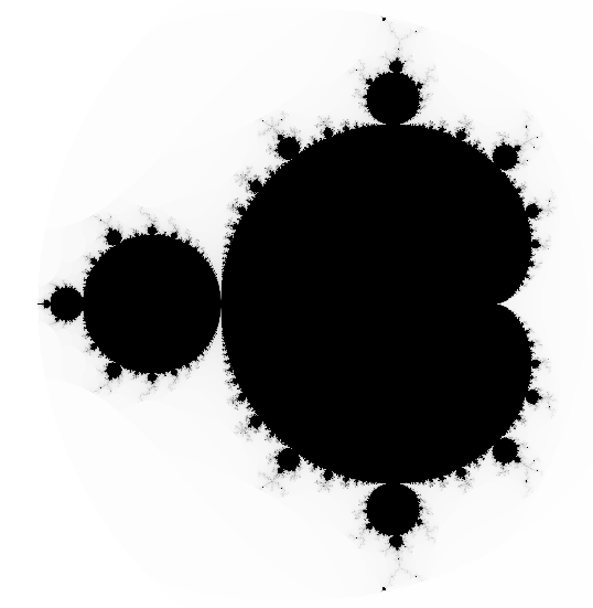
This clipping restriction isn't always necessary, and it might not be necessary for all points within a given figure, which raises an interesting prospect: What if we try to identify the points that fly off into infinity and those that don't?

check = Compile[{{c, _Complex, 0}},
   Module[{i = 0, z = 0 I},
    While[
     Abs[z] < Sqrt[2] && i++ < 240,
     z = z^2 + c];
    -i]];

ImageAdjust@Image@
  ParallelTable[check[x + y I],
   {y, -1.1, 1.1, .0035}, {x, -1.55, .6, .0035}]

vertices = (**)5(**) {Cos[#], Sin[#]} & /@ (2 Pi Range[3]/3);

check = Compile[{{x, _Real, 0}, {y, _Real, 0}},
   Module[{i, b, diff, z = {0., 0.}, vertices = vertices},
    Total@Table[
      i = 0; z = {x, y};
      While[z.z < 40 && i++ < 120,
       b = RandomChoice[vertices];
       diff = b - z;
       z = (z + b) Log[Sqrt[diff.diff] + .01]];
      -i,
      {20(*0*)(*number of trials*)}]]];

img = ImageAdjust@Image@
    ParallelTable[check[x, y],
     {y, -6.5, 6.5, .01}, {x, -6.5, 6.5, .01}];

img // Colorize // ImageResize[#, 550] &

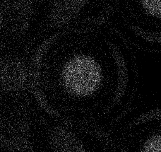
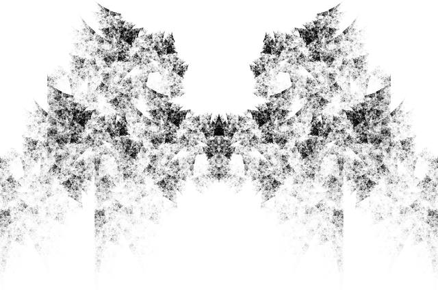
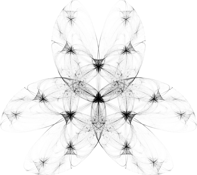
Here the white points go off into infinity quickly. The black points don't, or at least they take a lot longer to escape. There are certainly patterns here, but they're much less pronounced and computationally harder to reveal to than they are for the Mandelbrot set, which is the same idea for Julia iterations. But if you spin a few knobs you can find interesting figures irregardless. The different colors/shades are different escape speeds. It may not be immediately apparent, but these are fractals also.

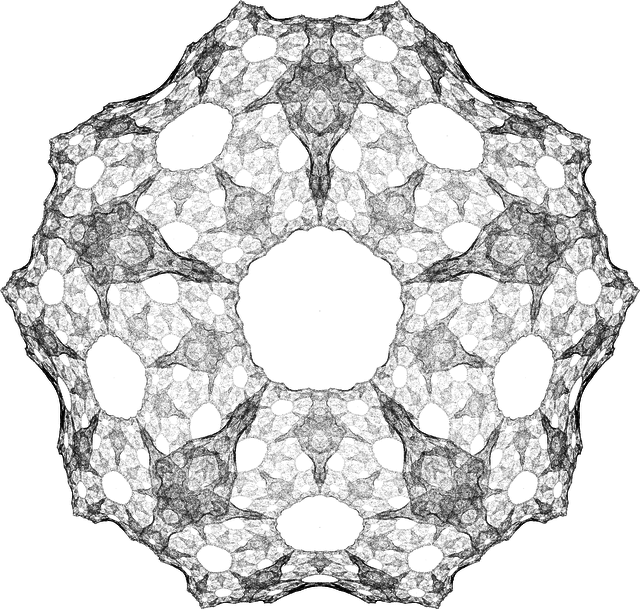
A lot of fractals have scaled/skewed characteristics, including the Mandelbrot set. I wonder if there's a non-trivial chaos game that can create the Mandelbrot set. Since we're skittering around complex numbers, is there an interesting complex-valued version of the logarithmic chaos game?

game = Compile[{{v, _Integer, 0}, {numPoints, _Integer, 0}},
   Module[{vertices},
    vertices =(*1.5*)E^(I 2 Pi Range[v]/v);

    FoldList[(*(Log[#1]+#2)/2&*)
     (#1 + (#1 + #2) Log[Sqrt[#2 - #1] + .7])/2.1 &, .1,
     RandomChoice[N@vertices, numPoints]]]];

Graphics[{Opacity[.1], PointSize[0],
  Point[{Im[#], Re[#]} & /@ game[2, 400000]]}]

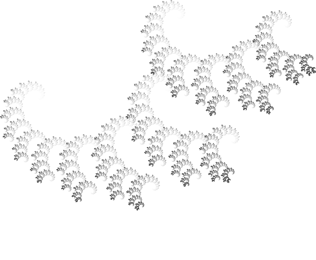
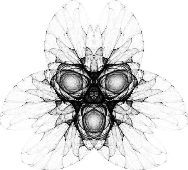
I don't know. Strictly speaking there wouldn't be a difference, but if you put on a blindfold and chuck logarithms at Mathematica helter-skelter, pretty pictures eventually come out. So I guess the answer is some form of yes. Formally these might still be considered Julia sets.

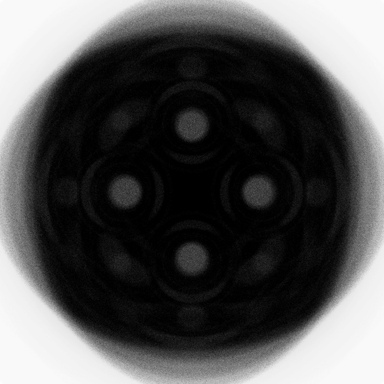
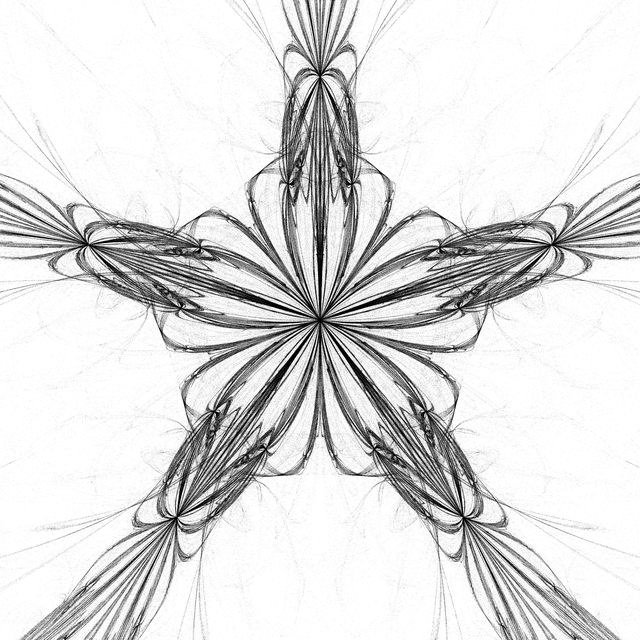
I've mentioned before that there are a lot of crazy distance functions out there for us to use in our chaos game, and there isn't anything special about the logarithm function. What do plots using other functions look like?

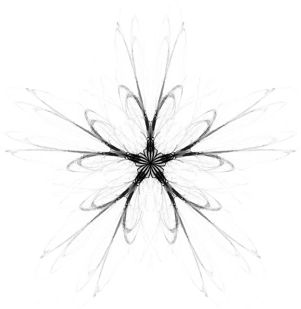
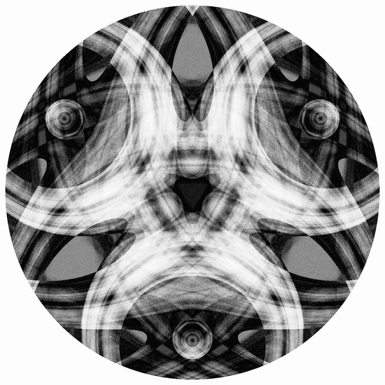
vertices = (**)5(**) {Cos[#], Sin[#]} & /@ (2 Pi Range[3]/3);

check = Compile[{{x, _Real, 0}, {y, _Real, 0}},
   Module[{i, b, diff, z = {0., 0.}, vertices = vertices},
    Total@Table[
      i = 0; z = {x, y};
      While[z.z < 40 && i++ < 120,
       b = RandomChoice[vertices];
       diff = b - z;
       z = (z + b) Sin[Sqrt[diff.diff] + .01]];
      -i,
      {20(*0*)(*number of trials*)}]]];

img = ImageAdjust@Image@
    ParallelTable[check[x, y],
     {y, -6.5, 6.5, .01}, {x, -6.5, 6.5, .01}];

img // Colorize // ImageAdjust // ColorConvert[#, "Grayscale"] & // ImageAdjust //
    ImageResize[#, Scaled[1/2]] & // ImageRotate[#, -Pi/2] & // ColorNegate //
 ImageApply[#^(1/1.3) &, #] &

game[f_, rest__] := rest //
   Compile[{{v, _Integer}, {w, _Real}, {numPoints, _Integer}, {rot, _Real}},
    Module[{diff, tmp, vertices},
     vertices = {Cos[#], Sin[#]} & /@ (rot + 2 Pi Range[v]/v);

     FoldList[(
        diff = #2 - #1;
        tmp = f[Sqrt[diff.diff] + w];
        Clip[(#1 + #2) tmp, 24 {-1, 1}]) &,
      {0, 0}, RandomChoice[vertices, numPoints]]]];

draw[{args__}, rot_: 0, options___] :=
  Graphics[{PointSize[0], Opacity[.25],
    Point[game[args, rot]]}, options];

draw[{Sin, 5, -1.23, 100000}, -Pi/10]
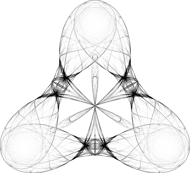
draw[{Cos, 3, Pi/2.675, 100000}, -Pi/6]
draw[{RamanujanTauL, 5, 3.1, 10000}, -Pi/10]

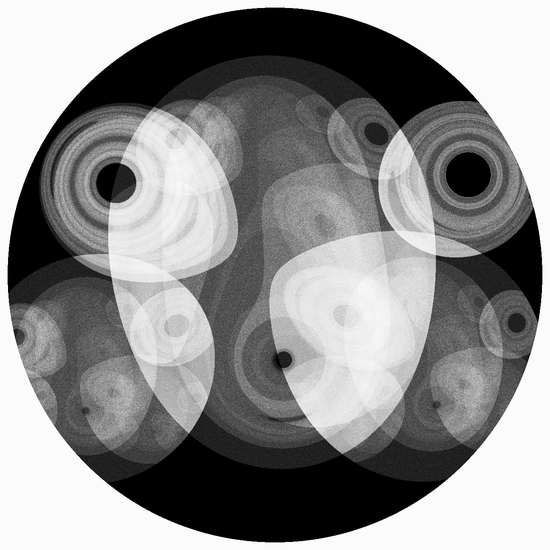
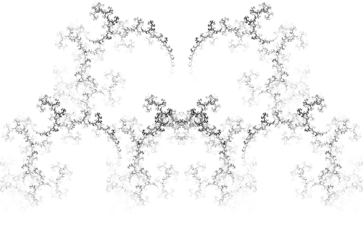
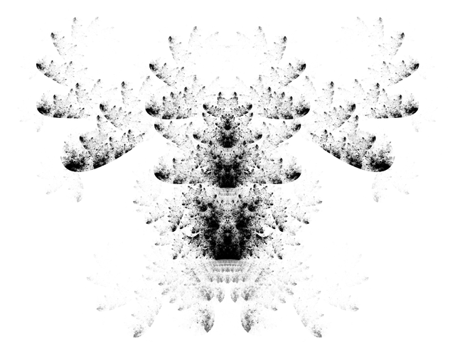
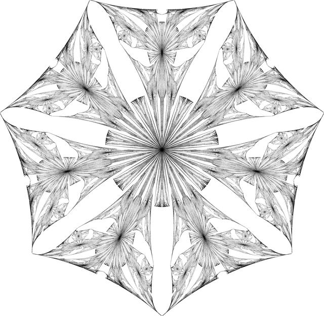
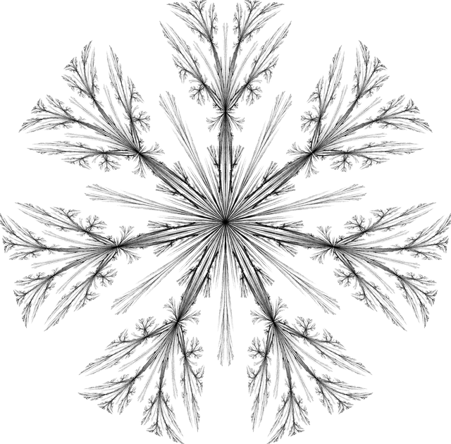
They look just as awesome, of course. Here we have plots using the sine, cosine, and, you guessed it, Ramanujan tau Dirichlet L-function. And this is using the same basic form as the logarithm version, without us even having to put on Loki's mask and get real buckwild. Speaking of masks.

Usually I don't pick favorites, but I like the cosine image (of course sin/cos are just offsets of eachother) because it has an infinite number of folded sheet things that seem to have precise contours. I'll leave the 3Dification as an exercise, but not the how-fast-points-go-to-infinity plot.

The reason it's easy to get all these pictures without trying very hard is that the self-similarity is almost guaranteed by the chaos game algorithm. As we saw earlier, "move toward a point" amounts to the same thing as "make a resized copy of everything toward the perspective of that point."

This is a simplification, but the point is that you essentially get the skeleton of self-similarity for free, or perhaps something a bit more broad. And more abstractly, I think some remarks could be made about the real number system itself.

What does the Sierpinski triangle sound like? One easy interpretation is to consider the L-system construction for the triangle and convert different angles to different frequencies as the turtle makes the triangle:

mp3 midi

mp3 midi

axiom = A;
rules = {A -> {B, R, A, R, B}, B -> {A, L, B, L, A}};
conversions = {A -> forward, B -> forward, L -> left, R -> right};

(*state transformations*)
forward[{z_, theta_}] := {z + E^(I theta), theta};
left[{z_, theta_}] := {z, theta + 2. Pi/6};
right[{z_, theta_}] := {z, theta - 2. Pi/6};

sier[n_] := Module[{program, zs},
   program = Flatten[Nest[# /. rules &, axiom, n]] /. conversions;
   zs = First /@ ComposeList[program, {0, 0}];
   First /@ Split[{Re[#], Im[#]} & /@ zs]];

(*convert angle into the given frequency range*)
freq[min_, max_][angle_] := angle (max - min)/Pi + min;

wave[coords_, dur_: 10, freq_: freq[6, 30]] := Module[{angles, freqs},
   angles = Abs[ArcTan @@@ Differences[coords]];
   freqs = Round /@ freq /@ angles;
   Sound[SoundNote /@ freqs, dur]];

wave[sier[3], 5, freq[8, 15]]

(*overtones zomg*)
Sound[{"NewAge",
  wave[#, {0, 20}] & /@ Table[
    RotationTransform[2 Pi i/4] /@ sier[i], {i, 4}]},
 SoundVolume -> .8]

It sounds totally lame. Not surprising since the L-system construction is simple. There is real power here though. This tonifier operates on coordinate lists of any kind, not just those produced by this particular L-system. And if you do things like layer different iterations on top of each other, you can get nifty chord thingies.

A variation of this would be to determine the waveform directly from the L-system. In a past life I made such a program in C#/WPF. It was around 1200 lines of code. In Mathematica it would be around 30 lines of code, and maybe around 150 lines total with a solid UI around it. It would also be about a million times more powerful/general/flexible. There's a lot of reasons for this, none of which have to do with math.

Luckily for me I don't have to explain. The goddess of finishing projects has finally crawled out of her cave and seen fit to smite her lightning bolt through my ears and across my temporal lobe, for this tune has sated and sedated the voices and quelled their cantankerous echoes. And so ends part 1.