Group Abstract Group Abstract

Message Boards Message Boards

0
|
121 Views
|
10 Replies
|
9 Total Likes
View groups...
Share
Share this post:

Trouble with scaling options in VectorPlot and StreamPlot

Posted 5 days ago

Several scaling options in VectorPlot and StreamPlot interact. I hope someone can explain the options so that I don't get the apparent contradiction in these plots.

POSTED BY: Jay Gourley
10 Replies

With my own old CurvesGraphics6 package we can easily draw stream lines onto the potential surface:

Module[{q1 = -0.5, q2 = 0.25, q3 = 0.74, potential},
 potential[x_, y_] = -(q1/EuclideanDistance[{x, y}, {1, 1}]) -
    q2/EuclideanDistance[{x, y}, {0, -1}] -
    q3/EuclideanDistance[{x, y}, {-1, 1}] /. Abs -> Identity;
 forceField[x_, y_] = D[potential[x, y], {{x, y}}];
 PlotCurveOnSurface3D[{{x, y, potential[x, y]},
   {x, -2, 2}, {y, -2, 2}},
  {forceField[x, y],
   {x, -2, 2}, {y, -2, 2},
   StreamColorFunctionScaling -> False}]]

stream plot on a surface

The package is available on my site.

POSTED BY: Gianluca Gorni

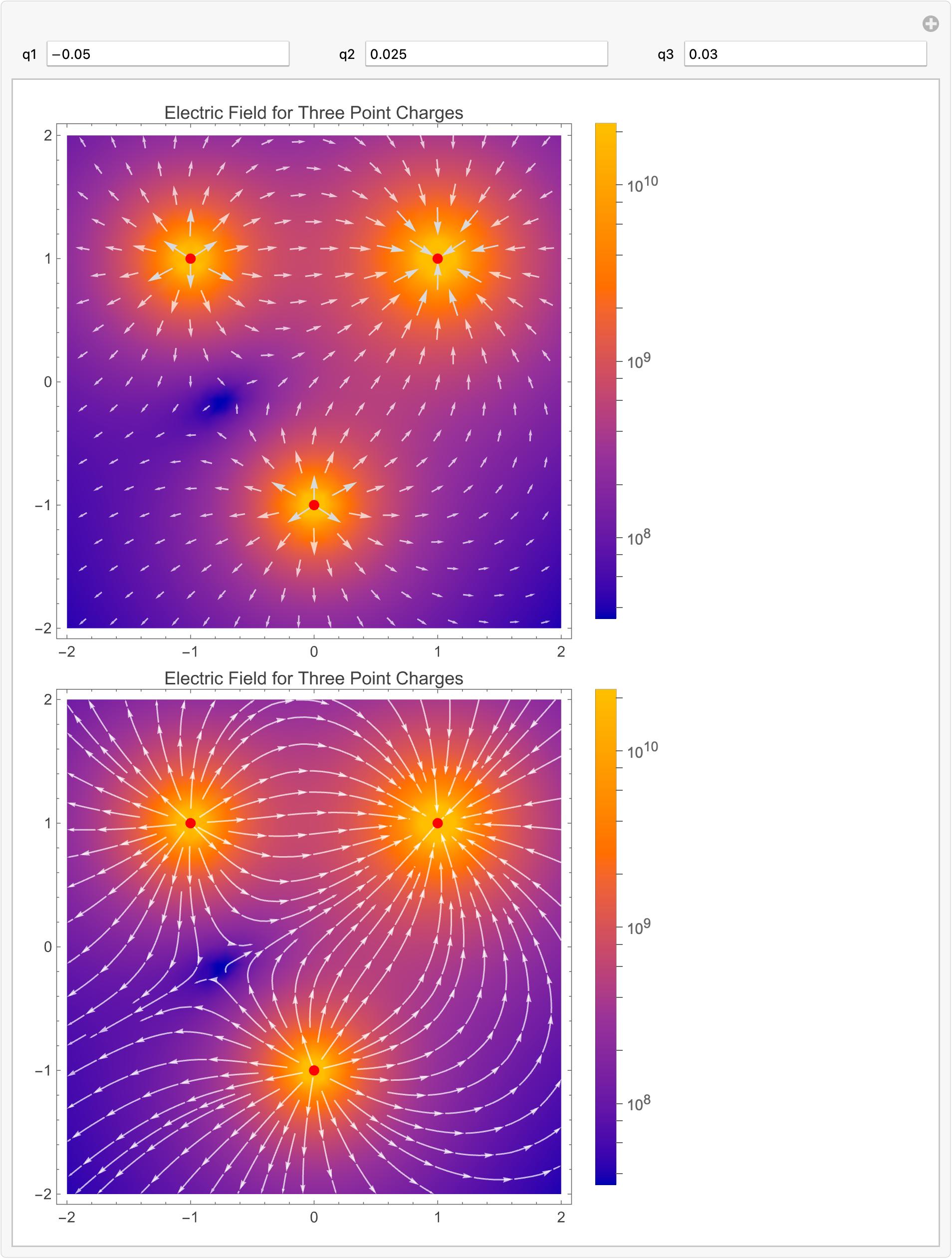
A different style, with the log of the field intensity as a background (just to give another idea about visualization; plus it was a bit harder to code than I thought it would be):

ClearAll[x, y, logTicks];
logTicks[{min_, max_}] := Replace[
   Range[Floor[min], Ceiling[max]],
   t1_List :> 
    Join[{#, 10^HoldForm[#]} & /@ t1, 
     Flatten[Table[{# + Log10@k, ""}, {k, 2, 8, 2}] & /@ Most@t1, 1]]
   ];
Manipulate[
 Module[{norm, q, field, \[Epsilon]₀(*,format*)(*,normRange*)},
  norm[vec_] := Sqrt[Total[vec^2]];
  q := {{q1, {1, 1}}, {q2, {0, -1}}, {q3, {-1, 1}}}; 
  \[Epsilon]₀ = 8.85418782 10^-12;
  field = 1/(4 \[Pi] \[Epsilon]₀ ) \!\(
\*UnderoverscriptBox[\(\[Sum]\), \(i = 1\), \(3\)]
\*FractionBox[\(q[[i, 1]]\ \(({x, y} - q[[i, 2]])\)\), 
SuperscriptBox[\(norm[{x, y} - q[[i, 2]]]\), \(3\)]]\);
  With[(* a bunch of nested With[]s *)
   {vplot = Reap[
      VectorPlot[field
       , {x, -2, 2}, {y, -2, 2}
       , VectorScaling -> Automatic
       , VectorColorFunction -> (GrayLevel[1., 0.7] &)
       , EvaluationMonitor :>(* sow norms to get range (below) *)
        Sow[Norm@field, "norm"]]
      , "norm"],
    splot = StreamPlot[field
      , {x, -2, 2}, {y, -2, 2}
      , StreamColorFunction -> (GrayLevel[1., 0.7] &)
      ]},
   {normRange = With[{
       bound = Block[{x, y},
         Max@Table[(* upper bound from offset of charged points *)
           {x, y} = q[[i, 2]] + {0.1, 0.1}; Norm[field]
           , {i, 3}]]},
      Log10@Clip[MinMax@{Last@vplot, bound}, {bound/10000., bound}]
      ]},
   {scf = 
     ColorDataFunction["WL12DefaultVectorGradient", 
        "ThemeGradients", {0, 1}, 
        Blend["WL12DefaultVectorGradient", #1] & ][
       Rescale[#1, normRange]] &},
   {leg = BarLegend[{scf, normRange}
      , ColorFunctionScaling -> False
      , Ticks -> logTicks[normRange]]},
   {format = {PlotLabel -> "Electric Field for Three Point Charges"
      , PlotLegends -> leg
      , Epilog -> {Red, PointSize[0.02`], 
        Table[Point[q[[i, 2]]], {i, 1, Length[q]}]}
      , ImageSize -> Medium}},
   {fieldStrength = DensityPlot[Norm@field, {x, -2, 2}, {y, -2, 2}
      , ColorFunctionScaling -> False
      , ColorFunction -> Function[{n}, scf[Clip[Log10@n, normRange]]]
      , PlotRange -> All
      , format (* needed only here b/c of Show[] *)
      ]},
   Column[
    {Show[fieldStrength, First@vplot, PlotLegends -> leg],
     Show[fieldStrength, splot, PlotLegends -> leg
      ]}
    ]
   ]],
 Row[
  {Control[{{q1, -0.05}, ControlType -> InputField}], Spacer[30],
   Control[{{q2, 0.025}, ControlType -> InputField}], Spacer[30],
   Control[{{q3, 0.03}, ControlType -> InputField}]}],
 TrackedSymbols :> Manipulate]

Manipulate output

POSTED BY: Michael Rogers

Is the problem limited to fields with holes?

I'd say that two independent plots are very likely to sample different points. If the norm does not change rapidly, then the color scale range of the two plots is likely to be similar, and the user is unlikely to notice the small difference in the coloring of the plot. If norm changes rapidly or through a few orders of magnitude, then the ranges of the norm at the sample points of each plot is likely to be different. This certainly happens near points where the norm goes to infinity ("holes", as you call them). Principle: Very large rate of change (derivative) times small difference in input => large difference in output.

Are such fields the motivation for StreamColorFunction?

Another use is to match a standard color scheme used in some field or other; or simply because users like their own color schemes. For instance, one might want to replicate the wind-velocity scale at the following site; also, it is absolute (equivalent to StreamColorFunctionScaling -> False) and not relative, so that colors are comparable from day to day:

https://earth.nullschool.net/#current/wind/isobaric/500hPa/orthographic

POSTED BY: Michael Rogers

Try setting VectorColorFunctionScaling -> False in the VectorPlot to match StreamColorFunctionScaling -> False in StreamPlot.

POSTED BY: Gianluca Gorni
Posted 4 days ago

Thanks, Gianluca Gorni. That brings the color scaling into conformity but the magnitudes of the vectors are still in conflict. I'm not sure either is correct. I couldn't post two versions in the same reply. So I'll reply again with a revised verstion.

POSTED BY: Jay Gourley

In StreamPlot the arrow heads are all of the same size, while in VectorPlot the heads follow the vector size. I don't understand why you see that as a conflict.

POSTED BY: Gianluca Gorni
Posted 4 days ago

I should have been more precise. The conflict I referred to is between values as shown in the legends. The extreme range in the streamplot version of the same vector field may be what accounts for the missing color range in the streams when color scaling was not disabled.

Michael Rogers later post identified the issue. The two vector field visualization functions have different sampling densities. So on a field like this with holes, StreamPlot with finer sampling picks up extreme values.

POSTED BY: Jay Gourley
Posted 4 days ago

Here's a link to a revised version. It executes on my local Windows Mathematica 14.3 but does not displayed in Wolfram cloud nor hereon the community website.

Attachments:
POSTED BY: Jay Gourley

The problem is that the range of the magnitude of the norm of the vectors is different in each plot. The sampling in the StreamPlot[] is much denser than the sampling in the VectorPlot[]. Since the norm of the vector goes to infinity near the q points, the sampling makes a big difference here. I think you need to do manual scaling of the color function, the same scaling for both plots. Something like:

StreamColorFunctionScaling -> False, 
StreamColorFunction -> Function[{x, y, vx, vy, n}, 
  ColorData["WL12DefaultVectorGradient"][
   Rescale[Clip[n, {0, 2.5*^10}], {0, 2.5*^10}]]]

This messes up the plot legends, though, and the documentation does not seem to suggest a way out. (It should, imo.) So here's a hack:

Manipulate[
 Column[
  Module[{norm, q, field, \[Epsilon]₀, format},
   norm[vec_] := Sqrt[Total[vec^2]];
   q := {{q1, {1, 1}}, {q2, {0, -1}}, {q3, {-1, 1}}}; 
   \[Epsilon]₀ = 8.85418782 10^-12;
   field = 1/(4 \[Pi] \[Epsilon]₀ ) \!\(
\*UnderoverscriptBox[\(\[Sum]\), \(i = 1\), \(3\)]
\*FractionBox[\(q[[i, 1]]\ \(({x, y} - q[[i, 2]])\)\), 
SuperscriptBox[\(norm[{x, y} - q[[i, 2]]]\), \(3\)]]\);
   format = {PlotLabel -> "Electric Field for Three Point Charges"
     , PlotLegends -> Automatic
     , Epilog -> {Red, PointSize[0.02`], 
       Table[Point[q[[i, 2]]], {i, 1, Length[q]}]}
     , ImageSize -> Medium};
   With[{vplot = 
      VectorPlot[field, {x, -2, 2}, {y, -2, 2}, 
       VectorScaling -> Automatic, Evaluate[format]]},
    {leg = Last@vplot},(* legend from vector plot *)
    {scf = leg[[1, 1, 1]], (* StreamColorFunction from vector plot *)
     normRange = leg[[1, 1, 2]]}, (* norm range from vector plot *)
    {vplot,
     StreamPlot[field
      , {x, -2, 2}, {y, -2, 2}
      , StreamColorFunctionScaling -> False
      , StreamColorFunction -> 
       Function[{x, y, vx, vy, n}, 
        scf[Rescale[Clip[n, normRange], normRange]]]
      , PlotLegends -> leg
      , Evaluate[format]]}
    ]
   ]],
 Row[
  {Control[{{q1, -0.05}, ControlType -> InputField}], Spacer[30],
   Control[{{q2, 0.025}, ControlType -> InputField}], Spacer[30],
   Control[{{q3, 0.03}, ControlType -> InputField}]}]]

I believe StreamPlot[] uses the vector field values at the beginning of a streamline arrow, where as VectorPlot[] uses the values at the middle of the vector arrow. Consequently, getting identical colors in both plots at the same points in the plane is a rather difficult battle to win. I imagine it could be done by post-processing the graphics.

POSTED BY: Michael Rogers
Posted 3 days ago

Thanks, Michael Rogers. That explains everything, colors, legends and all. I would never have figured that out on my own. This answers my original question, but I'll come back to this thread after I've tried your suggestion. I assume this problem affects all fields with holes. Is the problem limited to fields with holes? Are such fields the motivation for StreamColorFunction?

POSTED BY: Jay Gourley
Reply to this discussion
Community posts can be styled and formatted using the Markdown syntax.
Reply Preview
Attachments
Remove
or Discard