Group Abstract Group Abstract

Message Boards Message Boards

Predator Prey Plot over time

Posted 27 days ago

Hi;
I am trying to plot a progression of time periods for a Predator - Prey model using the function ParametricPlot with constants, Eigenvalues (raised to k powers and Eigenvectors - see attached notebook. However, I am having trouble getting any output. I am sure it is something that I am not coding correctly.

Thanks,
Mitch Sandlin

POSTED BY: Mitchell Sandlin
13 Replies

If we start with few foxes and many rabbits, fow a while the rabbits will increase. It will take time before the foxes catch up and they will both go extinct. Here is an example:

mat = {{6/10, 1/2}, {-(7/40), 6/5}};
f[t_] = MatrixPower[mat, t];
ParametricPlot[f[t] . {0, 1}, {t, 0, 30},
  PlotRange -> {{0, 2.1}, {0, 2}},
  AxesLabel -> {"foxes", "rabbits"}] /. Line -> Arrow

Using discrete steps:

mat = {{6/10, 1/2}, {-(7/40), 6/5}};
f[t_] = MatrixPower[mat, t];
pts = Table[f[t] . {0, 1}, {t, 0, 30}];
Graphics[{Arrowheads[{.05, .05, .05, .05}], Arrow[pts], 
  PointSize[Medium], Point[pts]}, PlotRange -> {{0, 2.1}, {0, 2}}, 
 Axes -> True, AxesLabel -> {"foxes", "rabbits"}]

Your initial picture only shows the regime where both decrease.

POSTED BY: Gianluca Gorni

Hi Gianluca;

I discovered that the key to getting what I wanted was using starting values that reflected the Eigenvalues. In the case of the attached Notebook, I used the exact Eigenvalues as the initial values.

I found it interesting that both your method and Eric's method produced exactly the same answer even though you used the MatrixPower function and Eric used Eigenvalues and Eigenvectors in his calculations.

Thanks so much, I not only obtained the answer, but learned a lot in the process.

Mitch Sandlin

Attachments:
POSTED BY: Mitchell Sandlin

Using MatrixPower:

mat = {{6/10, 1/2}, {-(7/40), 6/5}};
eigen = Eigenvectors[mat];
f[t_] = MatrixPower[mat, t];
ParametricPlot[{f[t] . {1, 1},
  f[t] . eigen[[1]], f[t] . eigen[[2]],
  f[t] . {1, 0}}, {t, 0, 20}] /. Line -> Arrow
POSTED BY: Gianluca Gorni

Another way:

mat = {{6/10, 1/2}, {-(7/40), 6/5}};
vel = D[MatrixPower[mat, t] . {x, y}, t] /. t -> 0
StreamPlot[vel, {x, -2, 2}, {y, -2, 2}]
POSTED BY: Gianluca Gorni
Posted 24 days ago

This is probably the nicest way to see the overall behavior of the system.

POSTED BY: Eric Rimbey

ParametricPlot[] is evaluated before the c's are replaced by numbers. You need to do the replacement first.

If f and r are scalars, then you're plotting a scalar, which ParametricPlot[] won't do.

If f and r are ordered pairs, then you're plotting an ordered pair, and you should see a plot, if the first point is addressed.

You can also use Unevaluated[] to address the first point:

Unevaluated[
  ParametricPlot[Subscript[c, 1]*(0.95^k*{10, 7} . {f, r}) + 
         Subscript[c, 2]*(0.85^k*{2, 1} . {f, r}), {k, 1, 10}]] /. 
   {Subscript[c, 1] -> 1, Subscript[c, 2] -> 1, f -> {1, -1}, 
     r -> {-3, 2}}

Oops, update: Just noticed the blackboard. I think one problem, which is addressed incorrectly in the 2nd and 3rd points, is that you should not be using . (Dot[]) in your code. The blackboard as scalar multiplication (* or Times[]), not vector-vector multiplication nor matrix-vector multiplication.

POSTED BY: Michael Rogers
Posted 27 days ago

Not quite sure of what you want, but if you want to see a preditor-prey population pair evolve over time, you can use ParametricPlot, yes. The whole eigenvector business is just turning the matrix arithmetic into scalar arithmetic, which means you can use a simple variable in your ParametricPlot.

Block[
 {k},
 With[
  {m = {{6/10, 1/2}, {-7/40, 6/5}}},
  {initialPopulations = {20, 50}},
  {es = Eigensystem[m]},
  {lc = SolveValues[k . es[[2]] == initialPopulations, k \[Element] Vectors[2, Reals]]},
  populationFn = Function[t, Total[es[[1]]^t lc[[1]] es[[2]]]]]]

Demonstration:

populationFn[6.5] // N
(* {80.7071, 69.0127} *)
(* about 81 foxes and about 69 rabbits *)

ParametricPlot[populationFn[t], {t, 0, 10}]
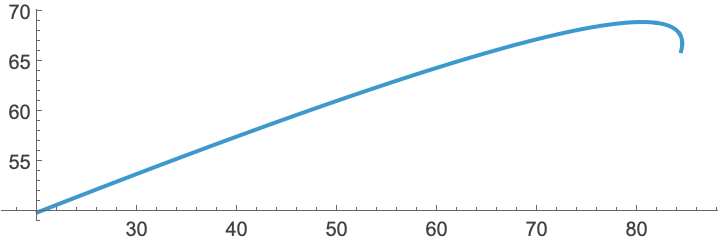
enter image description here

Explanation:

You don't necessarily need the Block, but I'm using the variable k in the Solve, and I just want to avoid a conflict.

The m is simply your predator-prey discrete dynamical system. initialPopulations is just an initial condition that I made up: 20 foxes and 50 rabbits. We need an initial value before we can solve for the linear combination of eigenvectors that we'll be using.

I'm using Eigensystem as a shortcut rather than calculating the eigenvectors and eigenvalues separately.

The lc is the linear combination of the eigenvectors that give the initial value.

The output is a function, and we can plug it into ParametricPlot. I'm just doing the standard arithmetic inside the Function. Note how we've moved from applying the matrix to do updates to just using scalars.

This doesn't look like the picture you posted, but I'm not sure what you were going for anyway. Ask follow ups if this doesn't help.

POSTED BY: Eric Rimbey

Hi Eric;

I find your response extremely interesting and am still studying your code to get a better understanding of your calculations. Additionally, I find your style of coding excellent since it is easy to read and understand.

Using your function "populationFn[6.5]" you calculated an approximate population of 81 Foxes and 61 Rabbits, and I was curious how you picked the time integral of 6.5.

Furthermore, the graph doesn't seem to model the expected outcome of the populations. For example, since both of the Eigenvalues are less than 1, one would expect both the Foxes and Rabbits to go extinct which the plot and the function do not demonstrate. Actually, it is my understanding that the populations should start decreasing immediately, as displayed in the graph that I attached in my original notebook, with the Rabbits going extinct first and then followed by the Foxes.

Since I am new at this and therefore could be incorrect, please review and give me your thoughts. In any event, I am a lot closer now thanks to you help.

Thanks Again,

Mitch Sandlin

POSTED BY: Mitchell Sandlin
Posted 24 days ago

how you picked the time integral of 6.5

I just made it up. I thought it would be interesting to see how the function is defined for non-integers, whereas the original system expects integer time intervals.

it is my understanding that the populations should start decreasing immediately

Well, you can just test that.

f[x_] := .6 f[x - 1] + .5 r[x - 1];
r[x_] := -.175 f[x - 1] + 1.2 r[x - 1];

(*initial conditions:*)
f[0] = 20;
r[0] = 50;

(*first generation:*)
{f[1], r[1]}
(* {37., 56.5} *)

Also, just look at the functions, for example f[x_] := .6 f[x - 1] + .5 r[x - 1]. That tells me that if the rabbit population is at least 80% of the fox population, then the fox population will go up.

But more abstractly, the sign of the eigenvalue doesn't really tell you much, because you could just take the negative and reverse the eigenvectors.

one would expect both the Foxes and Rabbits to go extinct

They do. Both populations start to decrease somewhere around the 9th generation, and things are looking pretty dire by 100 generations. :)

POSTED BY: Eric Rimbey

Hi Eric:

After spending a little time playing with the code, I realized that YOU NAILED IT! This is exactly what I wanted and a little more.

What I did, I changed the initial values to the Eigenvectors and got exactly what I was looking for. Additionally, Gianluca Gorni introduced another method using the function MatrixPower[] that gave the exact same answer which further verified the accuracy.

Thanks so much, I certainly appreciate your help,

Mitch Sandlin

Attachments:
POSTED BY: Mitchell Sandlin
Posted 21 days ago

Thanks! I'll just point out that Gianluca's method is basically the standard way you'd do this. The only reason to use linear combinations of eigenvectors is to turn matrix multiplication into scalar multiplication (which could give performance improvement). Given the way you set up your original problem, I thought that's what you wanted.

POSTED BY: Eric Rimbey

I am trying to guess what f and r may be:

With[{c1 = 1, c2 = 1, f = 1, r = 1},
 Plot[c1*0.95^k {10, 7} . {f, r} +
   c2*0.85^k {2, 1} . {f, r}, {k, 1, 10}]]
POSTED BY: Gianluca Gorni

Hi Gianluca;

In this predator - prey model, the f represents for "Foxes" and the r represents "Rabbits".

In the example that I submitted, I set the Predation value (the first value in the Rn+1 equation to - 0.175 which gives Eigenvalues of {.95, .85}. Since both these eigenvalues are less than 1 then over time both the Foxes and Rabbits should go extinct (as the provided graph in my attached notebook displays). My goal is to produce a plot to show this progression over several periods using Mathematica.

Thanks,

Mitch Sandlin

POSTED BY: Mitchell Sandlin
Reply to this discussion
Community posts can be styled and formatted using the Markdown syntax.
Reply Preview
Attachments
Remove
or Discard