I don't think you're doing anything wrong. TransformedDistribution just doesn't always find a result when there is a legitimate result. In that case one can try a brute force approach. (You probably already know how to do this and the following isn't the desired solution. I agree that I'd like to have Mathematica do all of the heavy lifting. without going to a brute force approach.)
One first notices that
$t=u-v$ takes on values from -2 to 2. Then find the pdf for
$t$. Then find the pdf for
$|t|$.
The usual technique for finding the pdf of the difference in two independent random variables is to appropriately integrate the product of the pdf's with
$x$ and
$t+x$.
pdf = (1 - x^2) 3/4;
integrand = pdf (pdf /. x -> z + x)
(* 9/16 (1 - x^2) (1 - (x + z)^2) *)
Now find the appropriate limits of integration for
$x$.
Reduce[{-1 < x < 1, -2 < t < 2, -1 < t + x < 1}, x]
(* (-2 < t <= 0 && -1 - t < x < 1) || (0 < t < 2 && -1 < x < 1 - t) *)
We see that for
$-2 < t \leq 0$, we integrate
$x$ from
$-1 - t$ to
$1$. When
$0 < t < 2$, then we integrate x from
$-1$ to
$1-t$.
pdfNeg = Integrate[integrand, {x, -1 - t, 1}, Assumptions -> -2 < z <= 0] // FullSimplify
(* 3/160 (2 + z)^3 (4 + (-6 + z) z) *)
pdfPos = Integrater=[integrand, {x, -1, 1 - t}, Assumptions -> 0 < z < 2] // FullSimplify
(* -(3/160) (-2 + z)^3 (4 + z (6 + z)) *)
If we replace
$t$ with -Abs[t] in pdfNeg and replace
$t$ with Abs[t] in pdfPos, we see that the resulting pdf values have the same form.
pdfNeg /. t -> -Abs[t] // FullSimplify
(* -(3/160) (-2 + Abs[t])^3 (4 + Abs[t] (6 + Abs[t])) *)
pdfPos /. t -> Abs[t] // FullSimplify
(* -(3/160) (-2 + Abs[t])^3 (4 + Abs[t] (6 + Abs[t])) *)
So the pdf of
$z=|t|$ is twice pdfPos with Abs[t] replaced with z. Simplified we have
pdf=(3/80) (2 - z)^3 (4 + z (6 + z))
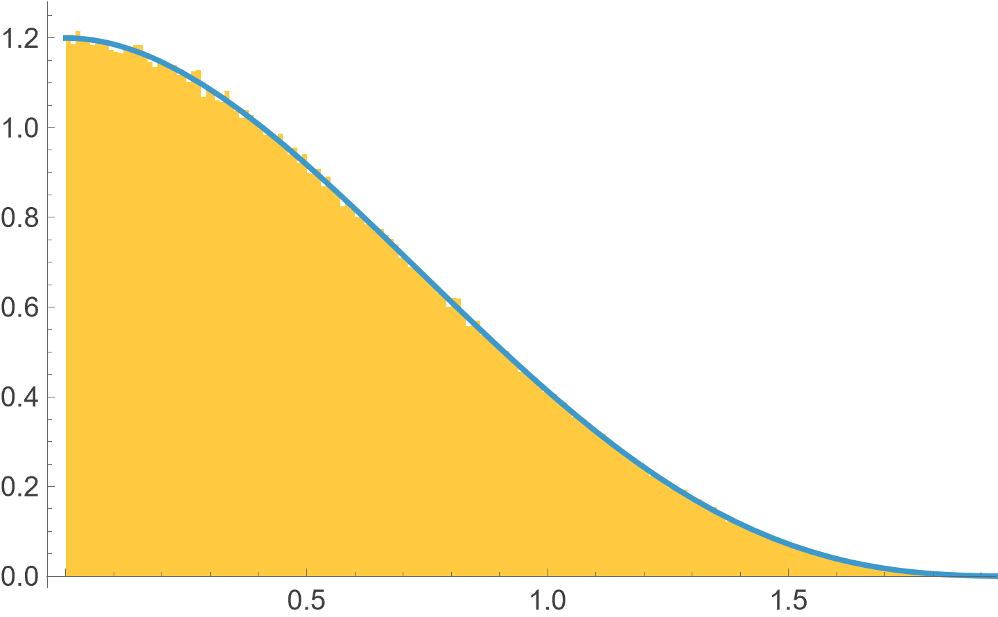
As a check consider the following.
f = TransformedDistribution[u^(1/3)*v, {u \[Distributed] UniformDistribution[{0, 1}], v \[Distributed] UniformDistribution[{-1, 1}]}];
w = RandomVariate[f, {1000000, 2}];
z = Abs[w[[All, 1]] - w[[All, 2]]];
Show[Histogram[z, "FreedmanDiaconis", "PDF"],
 Plot[3/80 (2 - z)^3 (4 + z (6 + z)), {z, 0, 2}]]