Introduction

Langton’s Ant is a simple mathematical model that produces surprisingly complex behavior. It was introduced by the scientist Chris Langton in 1986 and is often studied in the context of cellular automata.

The principle of Langton's Ant

Imagine an infinite white grid. Squares are colored either black or white. At each step, the ant can travel in any of the four cardinal directions by following two simple rules :

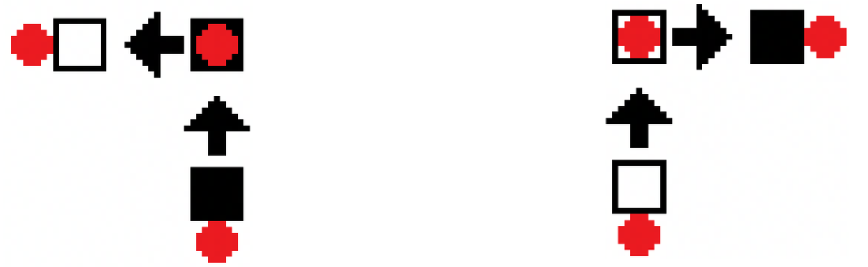
• At a white square, turn 90° clockwise, flip the color of the square, move forward one unit
• At a black square, turn 90° counter-clockwise, flip the color of the square, move forward one unit

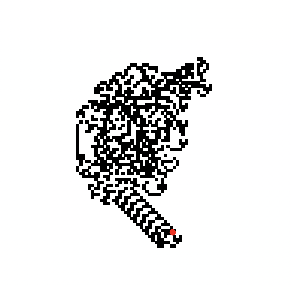
Despite these extremely simple rules, the ant’s behavior is fascinating. At first, its movement appears chaotic and unpredictable. However, after a certain number of steps, a clear pattern emerges: the ant starts building a regular repeating path called a “highway” that continues indefinitely. We don't fully understand Langton's ant behavior, and although every simulation of the original Langton's ant appears to end in a highway, no mathematical proof is currently known that this must always happen.

Basic Simulation with the Wolfram language

Our first step was to recreate Langton's ant ourselves. We created a single function named donutshaped[], so that it would be easier for us to manipulate Langton's Ant afterwards.

Here are the lines that permit us to set the environment : a grid where 0 represents a white cell and 1 represents a black cell. The first direction of the ant is chosen randomly.

side = 100;
grid = ConstantArray[0, {side, side}];
ant = {50, 50};
state = RandomChoice[{"right", "down", "left", "up"}];

This is the heart of the algorithm. The rule is based on the current state {color of the cell, direction} and the output gives {new color, new direction}.

ruleposition = {
   {1, "up"} -> {0, "left"},
   {1, "down"} -> {0, "right"},
   {1, "left"} -> {0, "down"},
   {1, "right"} -> {0, "up"},
   {0, "up"} -> {1, "right"},
   {0, "down"} -> {1, "left"},
   {0, "left"} -> {1, "up"},
   {0, "right"} -> {1, "down"}};

Once the rules are correctly set, we convert directions into movements. Note here that the grid is a matrix, and matrices are indexed from the top left corner, and its coordinates are based on rows and columns.

ruledir = {
   "up" -> {-1, 0},
   "down" -> {1, 0},
   "left" -> {0, -1},
   "right" -> {0, 1}};

Finally, here is our function step[] which updates, according to the rules that we saw, the movement of the ant and the color of the cell. We thought that a gigantic grid would slow down the algorithm and we wouldn't see the ant's movement. This is why we decided to make a toroidal grid, also called donut shaped grid.

step[] := Module[{color, res, move},
   color = grid[[ant[[1]], ant[[2]]]];

   res = {color, state} /. ruleposition;

   grid[[ant[[1]], ant[[2]]]] = res[[1]];
   state = res[[2]];

   move = state /. ruledir;
   ant = ant + move;
   ant = Mod[ant - 1, side] + 1;
   ];     (*This line makes the grid toroidal*)


  Dynamic[step[];
   ArrayPlot[Reverse[Transpose[grid]], ColorRules -> {0 -> White, 1 -> Black}, 
   Mesh -> False, Epilog -> {Red, PointSize[Medium], Point[ant + 0.5]}], 
   UpdateInterval -> 0]];

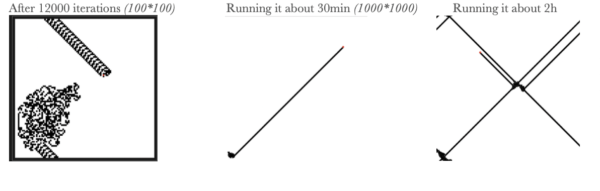
By executing our algorithm 5 times for about 1 hour for each run, we have indeed observed that once the ant begins its highway, it repeats its cycle indefinitely. We also observed that in a toroidal grid, all the highways that the ant makes are either parallel or perpendicular, as we can see on the last image. Additionally, we can also see that the highways are all diagonals of the grid.

Usually, Langton's ant moves on an "infinite" grid, or a toroidal grid. However, we decided to observe the behavior of the ant in a non toroidal grid, by setting boundaries. Here is our second algorithm non$donutshaped[], which is identical to the first algorithm, except that we set new rules : whenever the ant goes out of the grid, its coordinates are forced so that the ant remains in the grid.

rulewall = {
   p_ /; p[[1]] > side -> {{side, p[[2]]}, "up"},
   p_ /; p[[1]] < 1 -> {{1, p[[2]]}, "down"},
   p_ /; p[[2]] > side -> {{p[[1]], side}, "left"},
   p_ /; p[[2]] < 1 -> {{p[[1]], 1}, "right"},
   p_ :> {p, state}
   };

Finally, we replace the modulo rule, which is for the toroidal grid, by this :

verif = ant /. rulewall;
ant = verif[[1]];
etat = verif[[2]];

Timeline ----->

As we can see on the second image, in a non toroidal grid, the ant begins its highway just like in a toroidal grid. However, once the ant reaches a side of the grid, it starts erasing its own highway. It looks like the ant retraces its path in reverse, until making the grid all white again.

Fix a grid size S ∈ N. A state ω of Langton's ant consists of :

• a position (x,y) ∈ {0,…,N−1} ^2
• a direction d ∈ {0,1,2,3} (e.g. the variable etat)
• a configuration of the grid σ ∈ {0,1}^(N^2)

So there are :

Ω = {0,…,N−1}^2 * {0,1,2,3} * {0,1}^(N^2)

Ω= N^2 * 4 * 2^(N^2) states possible

Pigeonhole principle : Since Ω is finite, ∃ i < j such that ωi​=ωj​. Then : ω i+k = ω j+k ∀k≥0

Thus, we have a periodic system with period T = j - i

This is true no matter the boundary conditions. However, the value of T varies according to the type of the grid. In a non-toroidal grid, the walls create constraints on trajectories while the torus lets the ant "explore" more states before repeating. Thus, the period T is way shorter in a non toroidal grid, and we can rapidly see the cycle repeating itself.

However, we asked ourselves: why does the grid come back all white again with our algorithm? Periodicity means that we have a state that will repeat with a period T. Why is this state the white grid in our case ? We ended up having no real answer to it, we just convinced ourselves that we created a particular cycle.

Interactive Visualization

Langton's Ant highway is a pattern composed of 104 steps that repeats indefinitely. We wanted to be sure of that. However, our first algorithm is too fast to study step by step the ant's movement. Moreover, we realized that experimenting could be very time consuming without it depending on the number of steps needed. This is why we created another function, manipulate1ant[], which lets us manipulate multiple values.

To begin, we added SeedRandom[p]; and Button["Change initial direction", p = p + 1] in our Manipulate[] function. This lets us create a button which increments the p variable causing the initial direction to change since changing the value of p forces state = RandomChoice[{"right", "down", "left", "up"}]; to execute. Without SeedRandom[p]; the colored area would constantly turn. In addition, the n variable contains the number of steps which are executed thanks to Do[step[], {n}].

However, we needed ways to avoid crashing the code, so we decided to add a Max and Speed variable. The Max variable contains the maximum number of steps. This is useful since playing the ant's movement step by step is easier for smaller maximum values such as 1000 than bigger ones such as 11,000 or 100,000. Speed lets us modify the step interval of the slider.

Manipulate[
   SeedRandom[p];
   grid = ConstantArray[0, {Size, Size}];
   state = RandomChoice[{"right", "down", "left", "up"}];
   ant = {50, 50};

   step[] := Module[{color, res, move},
     color = grid[[ant[[2]], ant[[1]]]];
     res = {color, state} /. ruleposition;
     grid[[ant[[2]], ant[[1]]]] = res[[1]];
     state = res[[2]];
     move = state /. ruledir;
     ant = ant + move;
     ant = Mod[ant - 1, Size] + 1;];

   Do[step[], {n}];
   showGrid[], {{n, 0, "Number of steps"}, 0, Max, Speed, 
    Appearance -> "Labeled"}, {Max, 1000, 100000, 100}, {Speed, 1, 
    1001, 100}, Button["Reset", grid = ConstantArray[0, {Size, Size}];
    n = 0], Button["Change initial direction", p = p + 1]];

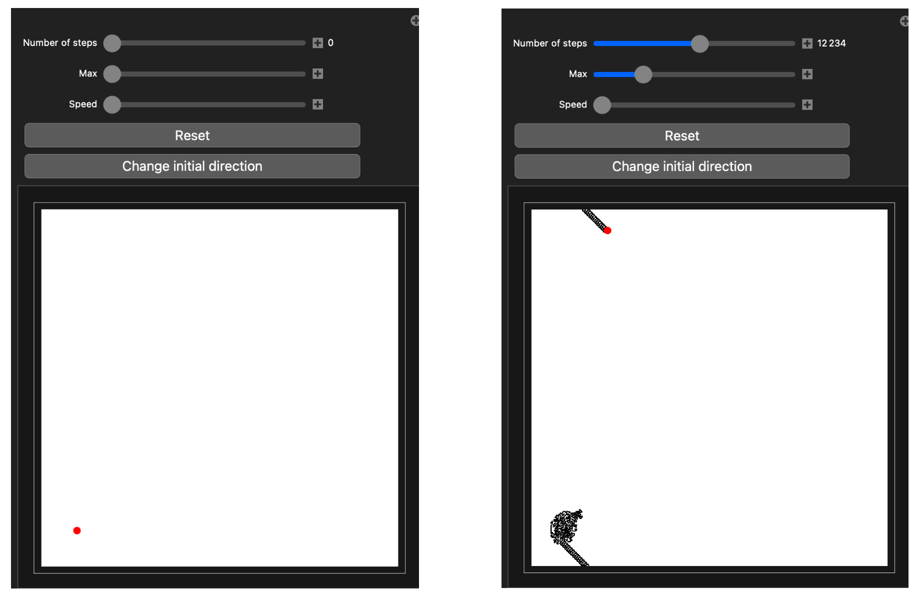
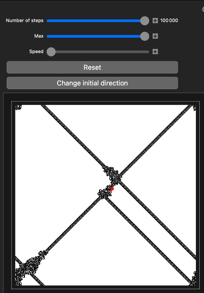
Thanks to our manipulate1ant[] function, we were able to observe more clearly the pattern.

Multiple Ants Case

We can easily think of putting multiple ants in one grid, to see how their behavior changes. The manipulate function allowed us to observe the movements in the Multiple Ants Case with greater speed and accuracy.

This meant that we needed to add more ways of manipulating the steps and positions of the ants. In addition we tripled the number of variables since each ant needed its own as you can see below.

 DynamicModule[{a, p, ruleposition, ant, ant2, ant3, position, 
  position2, position3, ruledir, state, state2, state3, ruleposition2,
  ruleposition3, showGrid, grid, step, step2, step3},

Moreover, we added 2 colors to distinguish each ant making each ruleposition 3 times bigger.

ruleposition = {{1, "up"} -> {0, "left"}, {1, "down"} -> {0, 
     "right"}, {1, "left"} -> {0, "down"}, {1, "right"} -> {0, "up"},
   {0, "up"} -> {1, "right"}, {0, "down"} -> {1, "left"}, {0, 
     "left"} -> {1, "up"}, {0, "right"} -> {1, "down"},
   {2, "up"} -> {0, "right"}, {2, "down"} -> {0, "left"}, {2, 
     "left"} -> {0, "up"}, {2, "right"} -> {0, "down"},
   {3, "up"} -> {0, "left"}, {3, "down"} -> {0, "right"}, {3, 
     "left"} -> {0, "down"}, {3, "right"} -> {0, "up"}};

The modified manipulate function lets the user control the 3 ants at the same time or each one separately. Do[step[], {n}]; Do[step2[], {s}]; Do[step3[], {t}]; Do[step[]; step2[]; step3[], {d}]; Each one of the letters n,s,t,d can be manipulated to customize the movements of the ants as desired. Such as: {{n, 0, "Number of steps (black ant)"}, 0, Max, Speed, Appearance -> "Labeled"}, {{s, 0, "Number of steps (blue ant)"}, 0, Max, Speed, Appearance -> "Labeled"}, {{t, 0, "Number of steps (green ant)"}, 0, Max, Speed, Appearance -> "Labeled"}, {{d, 0, "Move them simultaneously"}, 0, Max, Speed, Appearance -> "Labeled"} We also added two buttons:

• A button to randomize the initial position of the ants:

  Button["Change the initial positions", a = a + 1; SeedRandom[a];
   position = {RandomInteger[{5, Size - 10}], 
     RandomInteger[{5, Size - 10}]};
   position2 = {RandomInteger[{5, Size - 10}], 
     RandomInteger[{5, Size - 10}]};
   position3 = {RandomInteger[{5, Size - 10}], 
     RandomInteger[{5, Size - 10}]};],
  

• To avoid a bug we decided to center the ants whenever the size of the grid changes by using TrackingFunction. This is the button to center the ants: Button["Center the ants", position = {Size/2, Size/2}; position2 = {Size/2 - 2, Size/2}; position3 = {Size/2 + 2, Size/2}; n = 0; s = 0; t = 0; d = 0]

We noticed he importance of the initial orientations and positions of the ants. In fact, if they are close to each other from the beginning, the ants will collide before starting their highway and their interaction will completely change their trajectories. Here, the first highway appears at only 30000 steps (approximately).

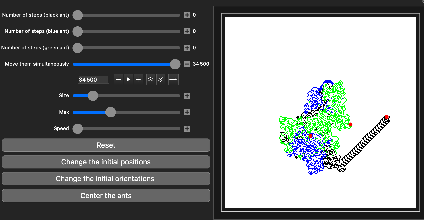
The collisions between two highways looks unpredictable:

• we observed cases where the highways were just crossing each other (for the second picture : the blue ant crossing with the green ant at the top left):

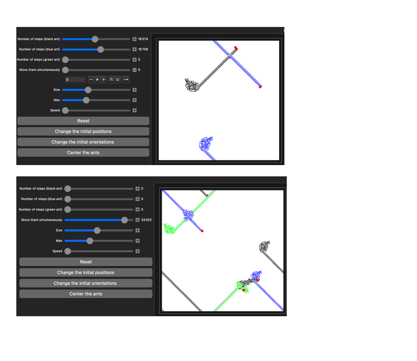
• but sometimes, we observed highways which "blocked" each other and didn't cross (1: the blue highway is being blocked by the black highway at the top right) / (2: the green is being blocked by the blue) :

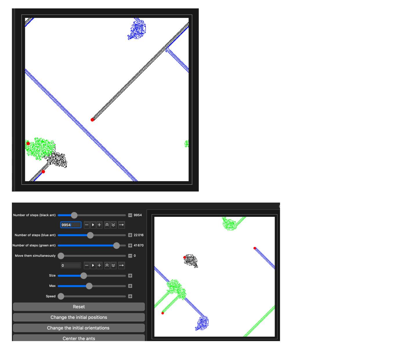
Finally, here is a very odd result : While the green ant is crossing the black ant's highway, the black ant is pursuing its highway around the blue ant's highway. In particular, we have this very odd pattern in the middle of the image made by the black ant just before starting its highway.

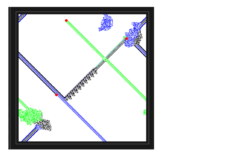
The multiple ants case was very surprising and we couldn't really deduce something from it. However, we conjectured that no matter the number of ants, if they are respecting the original rules of the game and have the required conditions, "the highway" will always appear. For example, one of the conditions is the size of the grid : the more ants added, the bigger the grid has to be to be able to create "the highway". ___

Tiling Variants

Triangular Tiling

The original Langton’s Ant operates on a square grid but we wondered how to make it in another shape grid.

The main challenge with this change is that the original version is working with ArrayPlot[], but this function only creates a grid of squares and after that it is really simple to change the colour of a single square.

Our solution was to create a “fake” grid compared to the original program. Its role is purely decorative and it is used only to represent the situation. We needed to model two types of triangles to make a tiling: those with a vertex pointing upward and those with a vertex pointing downward.

In the first part, we just create the two types of triangles with the function Polygon[] in which we define the 3 coordinates for each triangle. Everything in this part depends of lside and high. It allows us to create easily the switch between triangles.

lside = 1;
high = (Sqrt[3]/2)*lside;
triangles = 
 Flatten[Table[
   Module[{x = i*lside + Mod[j, 2] lside/2, 
     y = j*high}, {Polygon[{{x, y}, {x + lside, y}, {x + lside/2, 
        y + high}}], 
     Polygon[{{x, y}, {x + lside, y}, {x + lside/2, y - high}}]}], {j,
     0, 31}, {i, 0, 31}], 2];

After we set this grid, the only thing we do with it is display it in the last part of this program.

Row[{Graphics[{EdgeForm[Gray], FaceForm[White], triangles, Red, 
    PointSize[Medium], Point[ant], PointSize[Small], Black, way}, 
   ImageSize -> 250], Column[
   {
    "    Numbers of steps=", Dynamic[ste], 
    "   Numbers of black points=", Dynamic[Length@dicolor], 
    Dynamic[ListLinePlot[historique, 
      AxesLabel -> {"Steps", "Numbers of black points"}, 
      PlotRange -> All, ImageSize -> 400]]}]}]

However, this grid doesn’t allow us to directly change the color of the triangle when the ant passes on it. This is why we created a new list called dicolor. In the function step, dicolor checks if there is something associated with the current coordinates of the ant in the list. If there is nothing, it puts the coordinates into the list but if there is already something, it deletes it. In res, a coordinate in the list is associated with -1 and when there is nothing, res associates the number 1. -1 and 1 are corresponding to different colors (-1 -> Black, 1 -> White) .

step[] := (continue && (
     dicolor = 
      dicolor /. {_ /; MemberQ[dicolor, ant] -> 
         DeleteCases[dicolor, ant], _ -> Append[dicolor, ant]};

     res = ({MemberQ[dicolor, ant] /. {True -> -1, False -> 1}, 
         side}) /. ruleposition;

     side = res[[2]];

     move = side /. ruledir;
     ant = ant + move;
     ste = ste + 1;
     AppendTo[historique, Length[dicolor]]

     ));

The rules are obviously following the same method as before. We just need to change the values for the colors, and we also have to define the rules for the 6 directions : 3 for both triangles. Furthermore, the movements of the ant are now diagonals.

ruleposition = {
   {-1, "h1"} -> {1, "b3"},
   {-1, "h2"} -> {1, "b1"},
   {-1, "h3"} -> {1, "b2"},
   {-1, "b1"} -> {1, "h3"},
   {-1, "b2"} -> {1, "h1"},
   {-1, "b3"} -> {1, "h2"},
   {1, "h1"} -> {-1, "b2"},
   {1, "h2"} -> {-1, "b3"},
   {1, "h3"} -> {-1, "b1"},
    {1, "b1"} -> {-1, "h2"},
   {1, "b2"} -> {-1, "h3"},
   {1, "b3"} -> {-1, "h1"}};


ruledir = {
   "h1" -> {0, -Sqrt[3]/3},
   "h2" -> {1/2, Sqrt[3]/6},
   "h3" -> {-1/2, Sqrt[3]/6},
   "b1" -> {0, Sqrt[3]/3},
   "b2" -> {-1/2, -Sqrt[3]/6},
   "b3" -> {1/2, -Sqrt[3]/6}};

After a long runtime, the result looks different than the original version, there is not a chaotic period at the start and even if you wait a long time, you will not obtain a highway. We also can see that a certain shape is growing up after a lot of repetition of the program. Without the grid, the result is the same, that perfectly represents the decorative use of the grid in this algorithm.

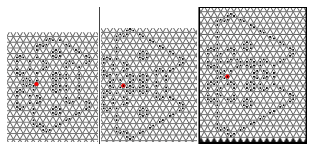
As the first direction is chosen randomly, we can have three different shapes possible. It is just the orientation of the shape that changes for example :

Hexagonal Tiling

Unlike what we did with the triangles (creating the shape vertex by vertex and repeat this method many times), this time we used RegularPolygon[] which allows us to create a shape of center {x,y} of radius r, with a certain number of sides. In this case, 6 sides.

radius = 1;
hexagones = 
 Table[{RegularPolygon[{x, y}, radius, 6], 
   RegularPolygon[{x + 1.5*radius, y + Sqrt[3]*radius/2}, radius, 
    6]}, {x, 0, 10, 3*radius}, {y, 0, 10, Sqrt[3]*radius}];

With this function, changing the size of the hexagon is very simple, we just have to change “radius”.

Additionally, to easily see beautiful creations, we added a checkbox to continue or not the program. The checkbox only changes the variable continue to true into false.

Once you have stopped the algorithm, you can always check again on the checkbox to continue the algorithm again.

step[] := (continue && (
...

For the direction rules, the angle of rotation is 60°. Of course, the changing of the position depends on the size of the shape.

ruledir = {
   "c1" -> {1.5, Sqrt[3]/2}*radius,
   "c2" -> {0, Sqrt[3]}*radius,
   "c3" -> {-1.5, Sqrt[3]/2}*radius,
   "c4" -> {-1.5, -Sqrt[3]/2}*radius,
   "c5" -> {0, -Sqrt[3]}*radius,
   "c6" -> {1.5, -Sqrt[3]/2}*radius};

The general rule is to divide 360 by the number of sides of the specific shape (120° for triangles, 90° for squares, 60° for hexagons, or 40° for enneagons). With this rule we can adapt Langton's ant to almost every shape and the ant only comes out from one of the nearest sides of the side it currently came from. Here is a basic explanation of by which side it can come out starting by the bottom side.

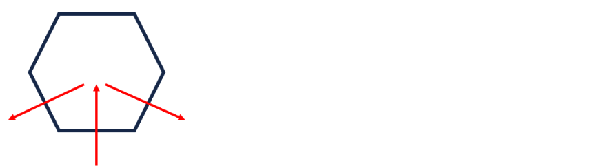
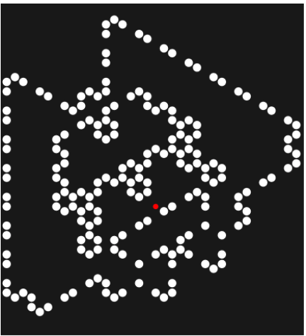
The result for the hexagons looks very similar to the evolution of the triangular tiling. We think that this similarity between triangles and hexagons comes from the fact that a hexagon is an assembly of 6 triangles.

Finally, to be sure of those new tilings, we decided to apply the hexagon's algorithm to the square, just by changing the positions and directions. The result was positive, the ant created a highway and had the same pattern as our first algorithm. ___

Quantitative Analysis

Number of black squares

We also thought that studying the behavior of the grid itself would be interesting. First, we decided to observe the number of black squares with our seventh function BlackBox[].

For our algorithm, we used the same principle as the one used for tiling variants. The key element is obviously dicolor which stores the coordinates of all the squares that are currently black. At every step, dicolor is being updated.

dicolor = 
  dicolor /. {_ /; MemberQ[dicolor, ant] -> 
     DeleteCases[dicolor, ant], _ -> Append[dicolor, ant]};

The variable history records the length of dicolor

AppendTo[history, Length[dicolor]

The function step[] is now finished, we just need to plot everything :

Row[{Graphics[{EdgeForm[Gray], FaceForm[White], square, Red, 
    PointSize[Medium], Point[ant], Black, path}, ImageSize -> 400], 
  Column[{"number of steps = ", Dynamic[stepCount], 
    "number of black points = ", Dynamic[Length@dicolor], 
    Dynamic[ListLinePlot[history, 
      AxesLabel -> {"Steps", "Number of black cells"}, 
      PlotRange -> All, ImageSize -> 400]]}]}]

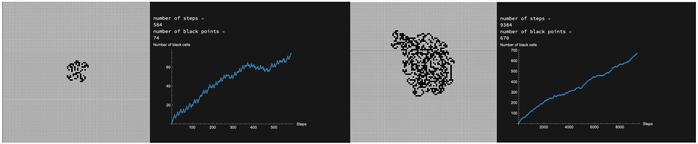
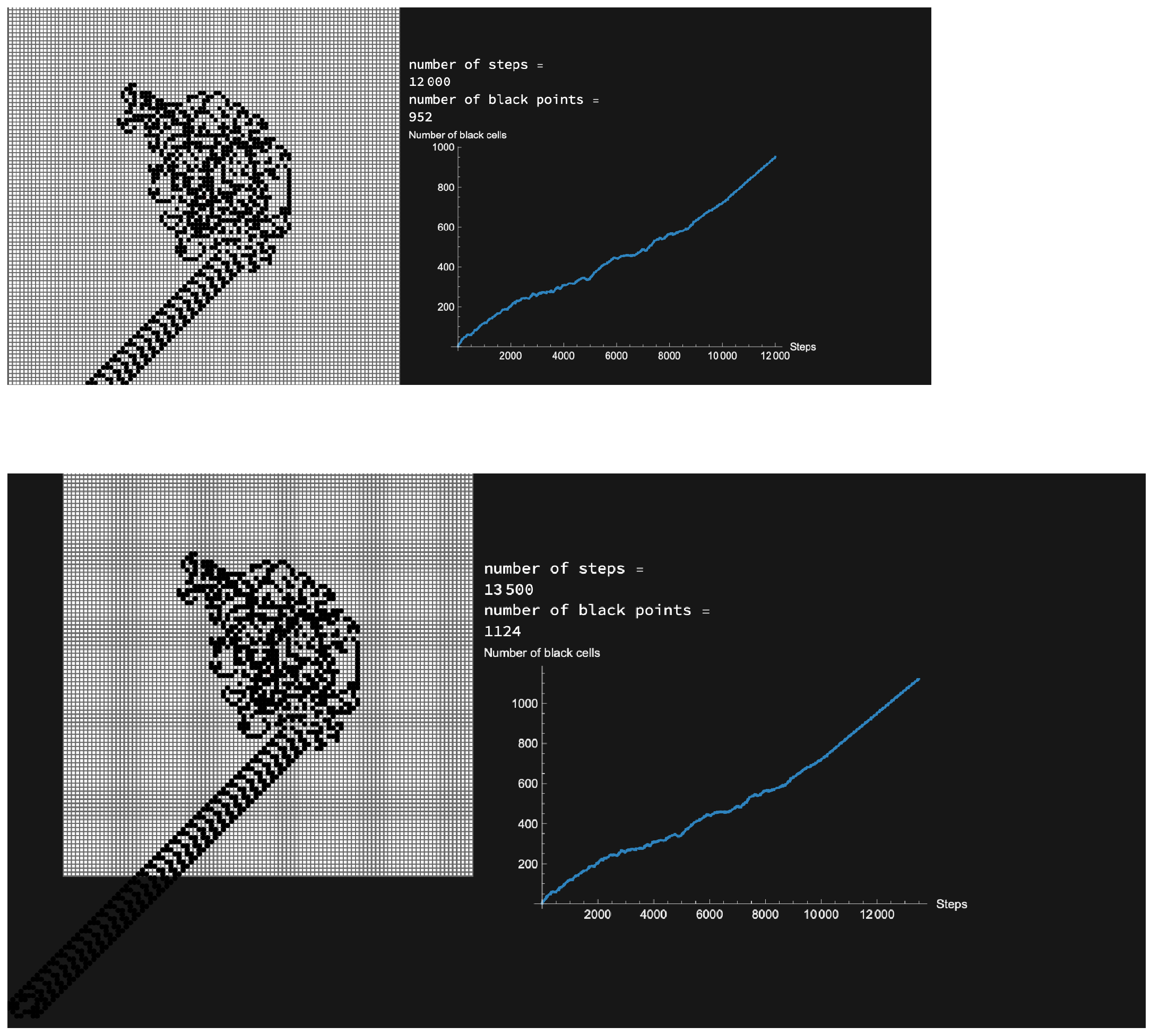
We observe a very intuitive result : at first, the behavior fluctuates, but then we see that the number of black squares increases steadily once the ant begins its highway. This graph shows well the periodicity of Langton's Ant.

Let B(n) be the sequence that associates the number of black squares with the number of steps. Over a large number of steps, we can pose B(n) ≈ an+b with n > 11000 (approximately).

From the two last pictures, we can calculate the average slope a of B(n):

(1124-952)/(13500-12000)​ = 43/375 ≈ 0.115

When the ant enters the highway phase, the number of black squares increases by roughly 0.115 black squares every step. The highway is constituted of cycles of 104 steps, so at each cycle, the ant is making approximately 43/375*104 ≈ 11.925 black squares.

We tried this algorithm with hexagons and triangles :

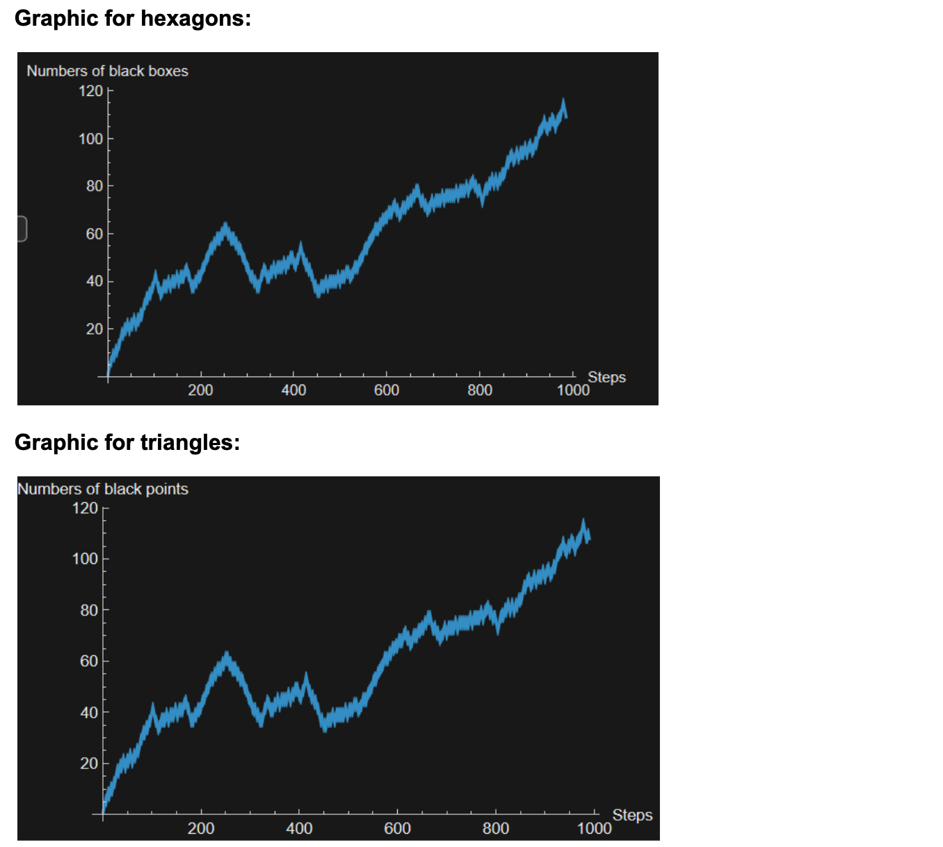
Here, the two graphics show well the similarity between triangles and hexagons. It looks even identical... we couldn't be really sure of that, but at first sight, there are no differences between those two graphics. We hope to dig more into this also.

Number of color switches

One square can change color several times. But how much ? And which squares in particular change the most ?

Therefore, we looked at the number of color switches for each squares thanks to our function BoxSwitches[]

Just like the variable history for the previous function, we created a variable counter that records the coordinates of the ant. By counting how many times each position appears, we know how many times each position's color changed. The algorithm shows the most visited cell and its number of changes by selecting the key associated with the highest value of Counts[Counter]. Additionally, this algorithm takes the 5 maximum number of changes, associated with the squares and make a bar chart of it.

Column[{"number of steps = ", Dynamic[stepCount], 
  "cell that changed the most = ", 
  Dynamic[First@
    Keys@Select[Counts[counter], # == Max[Values[Counts[counter]]] &]],
   "maximum number of changes = ", Dynamic[Max[Counts[counter]]], 
  Dynamic[BarChart[TakeLargest[Counts[counter], 5], 
    ChartLabels -> Automatic, ImageSize -> 400]]}]

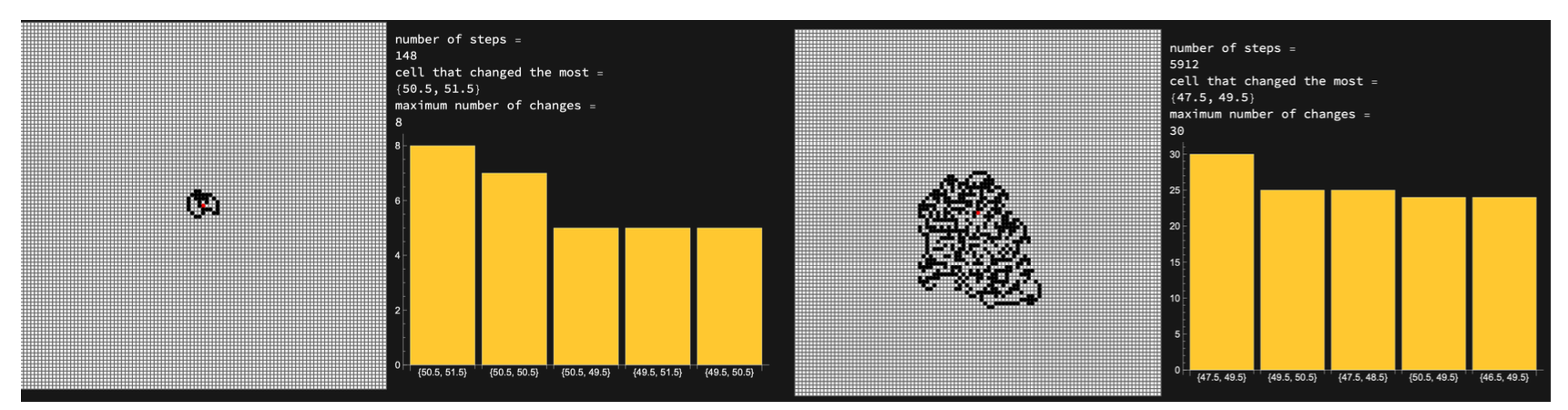
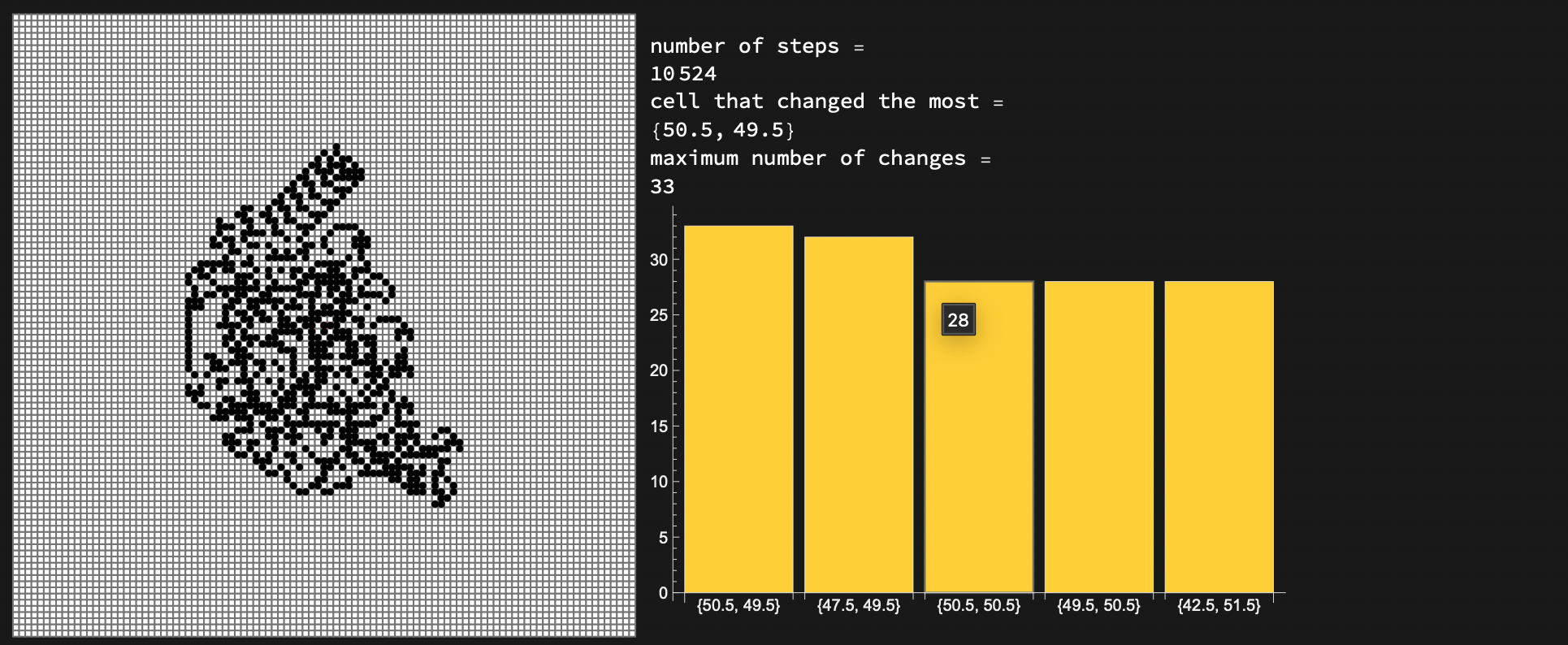
Here, the ant's starting point is {50.5,50.5}. After 5912 steps, we can see that the most visited box is {47.5,49.5}. We thought at first that the maximum number of changes stops growing at approximately 4000 steps (at 30 changes for the most visited square) because the ant is slowly distancing itself from the center. However, we can see that after 10 524 steps, the most visited box is {50.5,49.5} with 33 changes. We conclue that the ant goes back to the center before starting its highway.

Conclusion

This project's main goal was to make the algorithms and to discover Langton's ant thanks to the Wolfram Language, and in fact, it did allow us to understand Langton's Ant more deeply, which was something new for us. However, we know that our project is still very incomplete. In the future, we would like to dig more in what we started to explore, to prove and deduce more rigorously what we observed. Furthermore, we would also like to improve some of our functions, especially the ones on quantitative analysis, which are really time consuming. The graph and the grid are constantly updating at each step, which makes the algorithm slow and heavy.

We hope that our functions will help people interested in the subject, and entertain those who are curious.

Extension

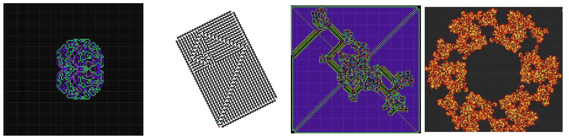
On the Wikipedia page, we can see some extensions of Langton's Ant. Extensions to multiple colors and to multiple states give impressive results, and we would like to dig deeper into it whenever we will have time.

Some Langton's Ant variations :

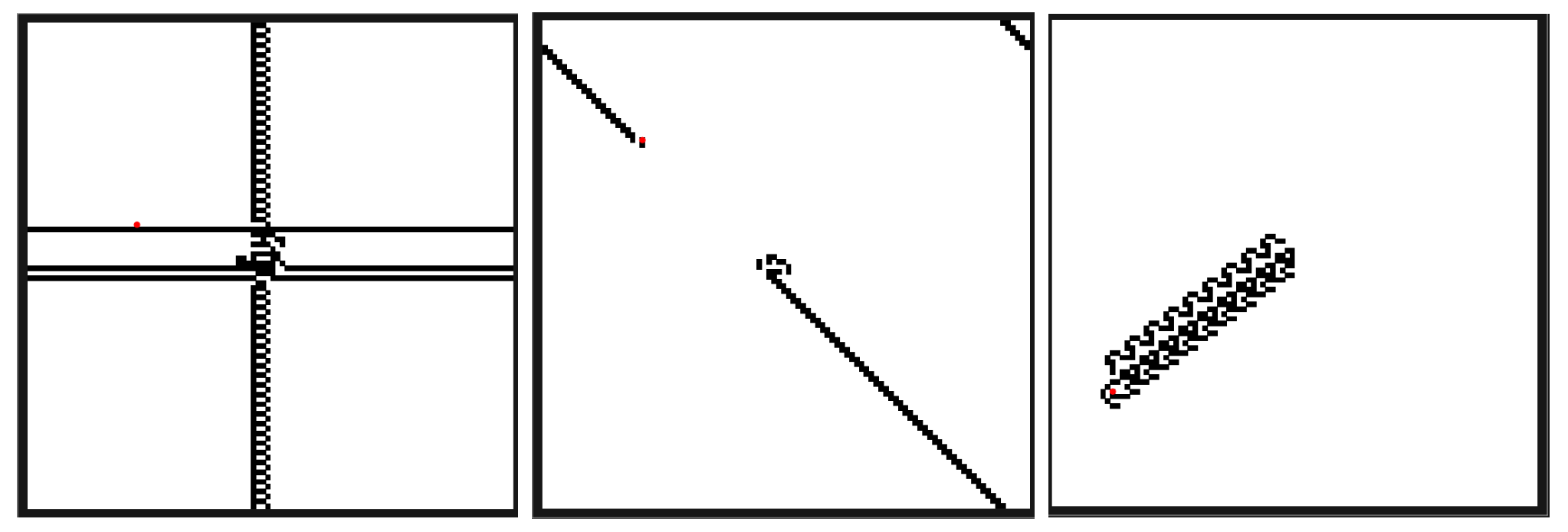
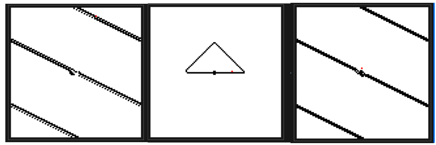
As a first step, we decided to play a little bit on the rules of our first algorithm, which already gave us some interesting variations. Here, we only changed the first rule : {1, "up"} -> {0, "left"} For example, the first image has {1, "right"} -> {0, "left"}:

Acknowledgements

This project was carried out during the Wolfram Language Summer School at Wolfram Research Europe. First of all, we would like to thank Victor-Emmanuel Dubau, our instructor who taught us from 0 the Wolfram Language with clarity and precision. We are also very grateful to Alexandre Upellini, who gave us the opportunity to attend this incredible summer school and who made sure to give us a comfortable and fun environment during those two weeks. Finally, we would also like to thank the speakers : Mario V., Maximilien Tirard, Joseph Brennan, Shadi Ashanti, Tom Wickham-Jones, Sophia Wolfram, and Ahmed E., who inspired us with their wonderful talks.

Attachments:

Quantitative analysis.nb

Tiling variants.nb

Toroidal & non t...nb

manipulate 1 ant...nb