Message Boards Message Boards

1
|
16285 Views
|
13 Replies
|
7 Total Likes
View groups...
Share
Share this post:

Plot pole and zero of transfer function in version 10.0

Posted 10 years ago

How to display pole and zero locations of transfer function without parameters, in version 8 there is RootLocusPlot command to Achieve this, but in version 10.0 it doesn't work without parameters and we should determine k parameter between kmin & kmax. Help me in version 10.0.

POSTED BY: Mehdi Rezai
13 Replies

Suba,

Thank you. I did not notice your use of PlotStyle->None. That does the trick!.

Yes, you can do something like the example above (which is already used in the documentation: Example 3 on the PoleZeroMarker Page) and make the Pole-Zero plot using your PlotStyle->None option:

RootLocusPlot[
 TransferFunctionModel[{{(k (10 + s^2))/(20 - 4 s + s^4)}}, s, 
  SamplingPeriod -> None, SystemsModelLabels -> None], {k, 0, 1}, 
 PlotStyle -> None, 
 PoleZeroMarkers -> {Style["\[Times]", 30], "", 
   Style["\[SmallCircle]", 40]}, PlotRange -> {{-2, 2}, {-6, 6}}]

Regards

POSTED BY: Neil Singer

Suba,

Thanks for the clarification. I think you should add an example of making an open loop pole zero plot to the RootLocusPlot documentation because there are a few subtle options that need to be set and explained:

  1. PoleZeroMarkers option takes a list of the {open-loop poles, closed-loop poles, open-loop zeros} and by putting "" for the closed loop poles, it no longer draws any closed loop poles.
  2. The value for k must be small so that the root locus that is drawn is not visible on the plot. In the example above, k=1 is small compared to the pole/zero values.

But in this documentation example, it would leave colored loci lines on the plot:

RootLocusPlot[
 TransferFunctionModel[{{(k (10 + s^2))/(20 - 4 s + s^4)}}, s, 
  SamplingPeriod -> None, SystemsModelLabels -> None], {k, 0, 1}, 
 PoleZeroMarkers -> {Style["\[Times]", 30], "", 
   Style["\[SmallCircle]", 40]}, PlotRange -> {{-2, 2}, {-6, 6}}]

enter image description here

Which can be removed with setting a tiny value for k:

RootLocusPlot[
 TransferFunctionModel[{{(k (10 + s^2))/(20 - 4 s + s^4)}}, s, 
  SamplingPeriod -> None, SystemsModelLabels -> None], {k, 0, 0.0001}, 
 PoleZeroMarkers -> {Style["\[Times]", 30], "", 
   Style["\[SmallCircle]", 40]}, PlotRange -> {{-2, 2}, {-6, 6}}]

To get:

enter image description here

Regards,

Neil

POSTED BY: Neil Singer
Posted 2 years ago

Neil,

  1. The behavior of "" is documented in a couple of places: https://reference.wolfram.com/language/ref/RootLocusPlot.html#1516150156 and https://reference.wolfram.com/language/ref/PoleZeroMarkers.html#991509519. I now think it may be a good idea to also add an example showing a pole-zero plot in the Properties and Relations section. Thanks for the suggestion.

  2. To make the loci invisible, add the option PlotStyle->None.

POSTED BY: Suba Thomas
Posted 2 years ago

Neil: The way to get RootLocusPlot to plot a pole-zero plot is the following.

RootLocusPlot[ k tfm3[s], {k, 0, 1}, 
 PoleZeroMarkers -> {Style["\[Times]", 30], "", 
   Style["\[SmallCircle]", 40]}, PlotStyle -> None, 
 PlotRange -> {Automatic, {-1000, 1000}}, AxesOrigin -> {0, 0}]

enter image description here

Koushik: The following should have worked, but it does not. This will directly change the size of the default markers. I will commit a fix for this.

Control`PoleZeroPlot[tfm3, 
 PoleZeroMarkers -> {{Automatic, 20}, {Automatic, 20}}, 
 PlotRange -> {Automatic, {-1000, 1000}}, AxesOrigin -> {0, 0}]

enter image description here

For now, the workaround is what Neil mentioned.

Control`PoleZeroPlot[tfm3, 
 PoleZeroMarkers -> {Style["\[Times]", 30], 
   Style["\[SmallCircle]", 40]}, 
 PlotRange -> {Automatic, {-1000, 1000}}, AxesOrigin -> {0, 0}]

enter image description here

POSTED BY: Suba Thomas

Dear Neil, Thank you so much for your kind help. Really appreciate this. I am learning. Regards, Koushik

Please format your code with the code sample button on the toolbar -- it makes it easier to read and to copy and paste.

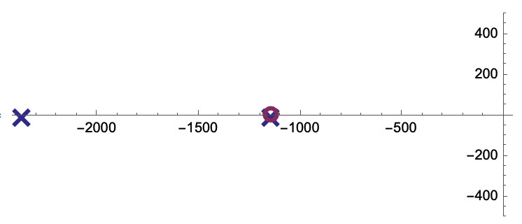
You need to use PoleZeroPlot with options -- you can't use inline notation (@). Using the code button :) it looks like this:

Control`PoleZeroPlot[tfm3, 
 PoleZeroMarkers -> {Style["\[Times]", 30], 
   Style["\[SmallCircle]", 40], Automatic}, 
 PlotRange -> {Automatic, {-500, 500}}, AxesOrigin -> {0, 0}]

You should play with the style values to get something that looks ok. This is a hard thing to plot because you have a zero and a pole in the same place so the plot does not look great.

enter image description here

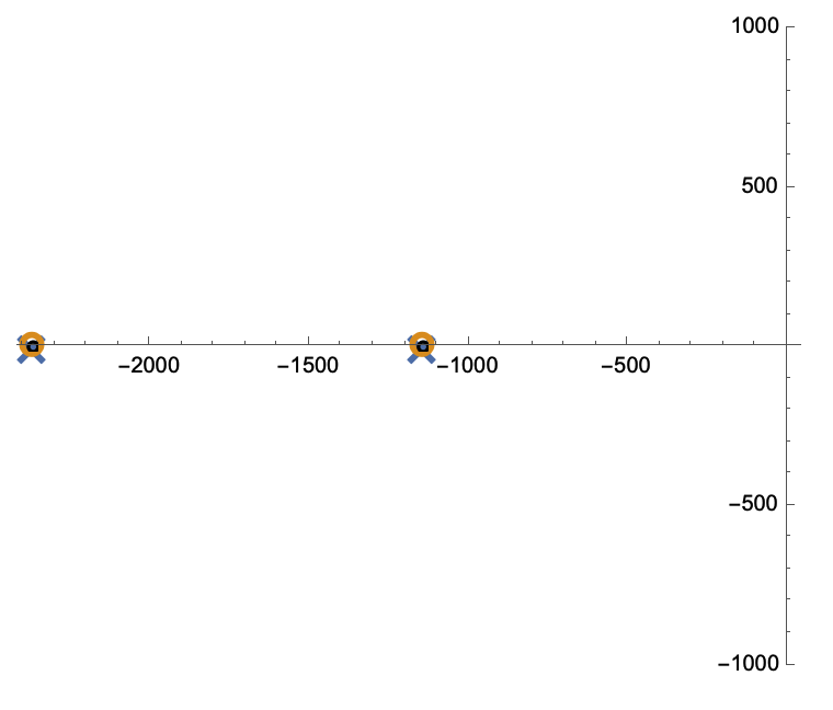
Normally, I would suggest that you do not use the unsupported/undocumented function and use RootLocusPlot instead:

RootLocusPlot[tfm3, {k, 0, 1}, FeedbackType -> None, 
 PoleZeroMarkers -> {Style["\[Times]", 30], 
   Style["\[SmallCircle]", 40], Automatic}, 
 PlotRange -> {Automatic, {-1000, 1000}}, AxesOrigin -> {0, 0}]

However, for some reason, it adds an extra zero on the plot. Maybe @Suba Thomas can explain what is happening here (Is it a bug??). if not, Suba, you should add an option to RootLocusPlot to just plot the open loop poles and an extra documentation example should be added to show how to make an open loop pole zero plot.

enter image description here

Lastly, another way to get publication quality plots exactly how you want them is to use TransferFunctionPoles and TransferFunctionZeros to get the poles and zeros and plot them using ListPlot and set various options to get exactly what you want (although this involves more effort in setting every option).

Regards,

Neil

POSTED BY: Neil Singer

Thanks but since I am new I am struggling a bit in understanding the syntax. Here is the transfer function for which I want to plot the pole-zero where the pole-zero markers need to be of publication standard:

tfm3 = TransferFunctionModel[{(
    1.3865251545716466`*^6 + 1215.0862273384766` s)/(
    2.699763486282365`*^6 + 3507.041473057938` s + 1.` s^2)}, s];

Using p2 = Control`PoleZeroPlot@tfm2 I am indeed getting the required pole-zero (as their traditional "x" and "o" marking symbol but they are really tiny. I need to make them bigger so that one can clearly see that one pole coincides with the zero.
As suggested, I tried to use the PoleZeroMarkers command but the problem is here we are using two different symbols to designate poles are zeros. Therefore it is not working as I wanted. I'll appreciate any solution.
Thanks.

You can use the same options as RootLocusPlot:

PoleZeroMarkers -> {Style["T", Large, Background -> Pink]}

Regards

POSTED BY: Neil Singer

Hi Suba, This command is great but how can I increase the size of the markers? Thanks. Koushik

Posted 10 years ago

You can also use Control`PoleZeroPlot.

Control`PoleZeroPlot@ButterworthFilterModel[12]

enter image description here

POSTED BY: Suba Thomas

OMG, that comand is awesone, but please, coud you explain the sintax, im new so i dont know from where this function comes or how it does to plot the things wih those markers

Posted 2 years ago

This is an undocumented function, but it's very straightforward. Given a TransferFunctionModel tfm, its pole zero plot can be obtained as

Control`PoleZeroPlot[tfm]

You are probably confused with the prefix operator @.

Control`PoleZeroPlot@tfm

also gives the same result.

POSTED BY: Suba Thomas
Posted 10 years ago

You can make the parameter a dummy -- it does not have to appear in the transfer function. The most confusing thing is that by default RootLocusPlot assumes a negative feedback loop around the transfer function. For me, by the time I want to do a root locus plot I have already developed the closed loop transfer function. So I set the FeedbackType to None.

tf = TransferFunctionModel[{{{{-40}}}, {{{-5 - 10 I, -5 + 
        10 I, -20}}}, {{1}}}, s];

RootLocusPlot[tf, {k, 0, 1}, FeedbackType -> None]
POSTED BY: David Keith
Reply to this discussion
Community posts can be styled and formatted using the Markdown syntax.
Reply Preview
Attachments
Remove
or Discard

Group Abstract Group Abstract