Message Boards Message Boards

0
|
9404 Views
|
3 Replies
|
0 Total Likes
View groups...
Share
Share this post:

How to solve 2-D Laplace equation in a rectangular domain analytically?

Posted 10 years ago

Hi everybody, I want to find an analytic solution for the 2-D Laplace equation in a rectangular domain. I've already found a numeric solution and I want to compare it with this one. I tried unsuccessfully to find a particular solution with DSolve and DSolveValue in the boundary conditions. I can only find the general solution for the PDE in C[1] and C[2]. I tried also to set up a system with boundary conditions and to Solve that in C[1],C[2] with no success. Could someone help me please? Thank you in advance. Here's my trial codes:

Clear["Global`*"];
Needs["DifferentialEquations`InterpolatingFunctionAnatomy`"];
DSolveValue[{D[u[x, y], {x, 2}] + D[u[x, y], {y, 2}] == 0, 
  u[x, 0] == 0, u[x, 20] == 2, u[0, y] == 0, u[20, y] == 1}, {u[x, y],
   u[x, y]}, {x, y}]

    Clear["Global`*"];
    Needs["DifferentialEquations`InterpolatingFunctionAnatomy`"];
    DSolveValue[{D[u[x, y], {x, 2}] + D[u[x, y], {y, 2}] == 0, 
      u[x, 0] == 0, u[x, 20] == 2, u[0, y] == 0, u[20, y] == 1}, {u[x, y],
       u[x, y]}, {x, y}]

Clear["Global`*"];
LaplaceEquation2D = {D[u[x, y], {x, 2}] + D[u[x, y], {y, 2}] == 0}
DSolve[LaplaceEquation2D, {u[x, y], u[x, y]}, {x, y}]
Solve[{C[1][I x + 0] + C[2][-I x + 0] == 0, 
  C[1][I x + 20] + C[2][-I x + 20] == 2, 
  C[1][I 0 + y] + C[2][-I 0 + y] == 0, 
  C[1][I 20 + y] + C[2][-I 20 + y] == 1}, {C[1], C[2]}]

Regards, Filippo

POSTED BY: Phil R
3 Replies

You can find separable solution with u[x,y]=f[x] g[y]

In[1]:= DSolve[{D[f[x], {x, 2}] == k, f[0] == 0, f[20] == 1}, f[x], x]

Out[1]= {{f[x] -> 1/20 (x - 200 k x + 10 k x^2)}}

In[2]:= DSolve[{D[g[y], {y, 2}] == -k, g[0] == 0, g[20] == 2}, g[y], y]

Out[2]= {{g[y] -> 1/10 (y + 100 k y - 5 k y^2)}}
POSTED BY: S M Blinder

Correction:

In[3]:= DSolve[{D[f[x], {x, 2}]/f[x] == k, f[0] == 0, f[20] == 1}, 
 f[x], x]

Out[3]= {{f[x] -> (
   E^(20 Sqrt[k] - Sqrt[k] x) (-1 + E^(2 Sqrt[k] x)))/(-1 + E^(
    40 Sqrt[k]))}}

In[4]:= DSolve[{D[g[y], {y, 2}]/g[y] == -k, g[0] == 0, g[20] == 2}, 
 g[y], y]

Out[4]= {{g[y] -> 2 Csc[20 Sqrt[k]] Sin[Sqrt[k] y]}}
POSTED BY: S M Blinder
Posted 10 years ago

Thank you S M Blinder. Ok now I can solve the equation, but when i plot the result, it is totally different from which I obtain with NDSolveValue. What do you think about? Thank you

Clear["Global`*"];
Needs["DifferentialEquations`InterpolatingFunctionAnatomy`"];
LaplaceEquation2D = {D[u[x, y], {x, 2}] + D[u[x, y], {y, 2}] == 0}
Xm = DSolve[{D[X[x], {x, 2}]/X[x] == 1, X[0] == 0, X[20] == 1}, X[x], 
  x]
Ym = DSolve[{D[Y[y], {y, 2}]/Y[y] == -1, Y[0] == 0, Y[20] == 2}, Y[y],
   y]
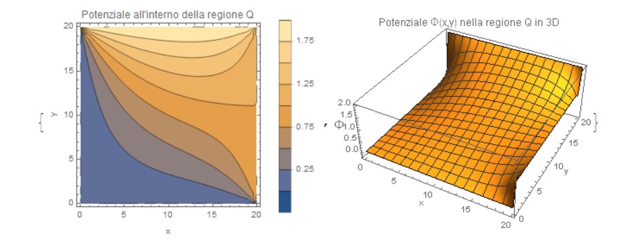
u[x, y] = (X[x] /. Xm)*(Y[y] /. Ym);
{ContourPlot[Evaluate[u[x, y]], {x, 0, 20}, {y, 0, 20}, 
  FrameLabel -> {"x", "y"},
  PlotLabel -> "Potenziale all'interno della regione Q", 
  ImageSize -> 250,
  PlotLegends -> Automatic],
 Plot3D[Evaluate[u[x, y]] , {x, 0, 20}, {y, 0, 20}, ImageSize -> 300, 
  AxesLabel -> {"x", "y", Style["\[CapitalPhi]", 15]}, 
  PlotLabel -> 
   Style["Potenziale \[CapitalPhi](x,y) nella regione Q in 3D", 12]]}

enter image description here

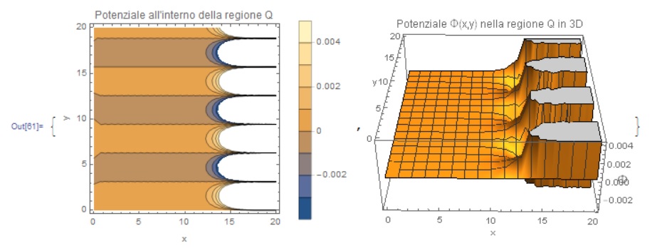
uval = NDSolveValue[{D[u[x, y], {x, 2}] + D[u[x, y], {y, 2}] == 0, 
   u[x, 0] == 0, u[x, 20] == 2, u[0, y] == 0, u[20, y] == 1}, 
  u, {x, 0, 20}, {y, 0, 20}]
{ContourPlot[uval[x, y], {x, 0, 20}, {y, 0, 20}, 
  FrameLabel -> {"x", "y"},
  PlotLabel -> "Potenziale all'interno della regione Q", 
  ImageSize -> 250,
  PlotLegends -> Automatic],
 Plot3D[uval[x, y] , {x, 0, 20}, {y, 0, 20}, ImageSize -> 300, 
  AxesLabel -> {"x", "y", Style["\[CapitalPhi]", 15]}, 
  PlotLabel -> 
   Style["Potenziale \[CapitalPhi](x,y) nella regione Q in 3D", 12]]}

enter image description here

POSTED BY: Phil R
Reply to this discussion
Community posts can be styled and formatted using the Markdown syntax.
Reply Preview
Attachments
Remove
or Discard

Group Abstract Group Abstract