Hello Wolfram Community! I am Fred Hohman, a senior Mathematics and Physics student at the University of Georgia. I have been working under Dr. David Gay in the Department of Mathematics at the University of Georgia since the beginning of the year, and I will be continuing my work until my graduation in May 2015.

Earlier in the summer I had the wonderful opportunity to meet Dr. Laura Taalman (mathgrrl) after her talk at MoMath on “Making Mathematics Real: Knot Theory, Experimental Mathematics, and 3D Printing.“ After chatting about math and 3D printing she asked me to say some words about my undergraduate research at UGA. Since I wrote my code in Mathematica I thought I would share the information here as well.

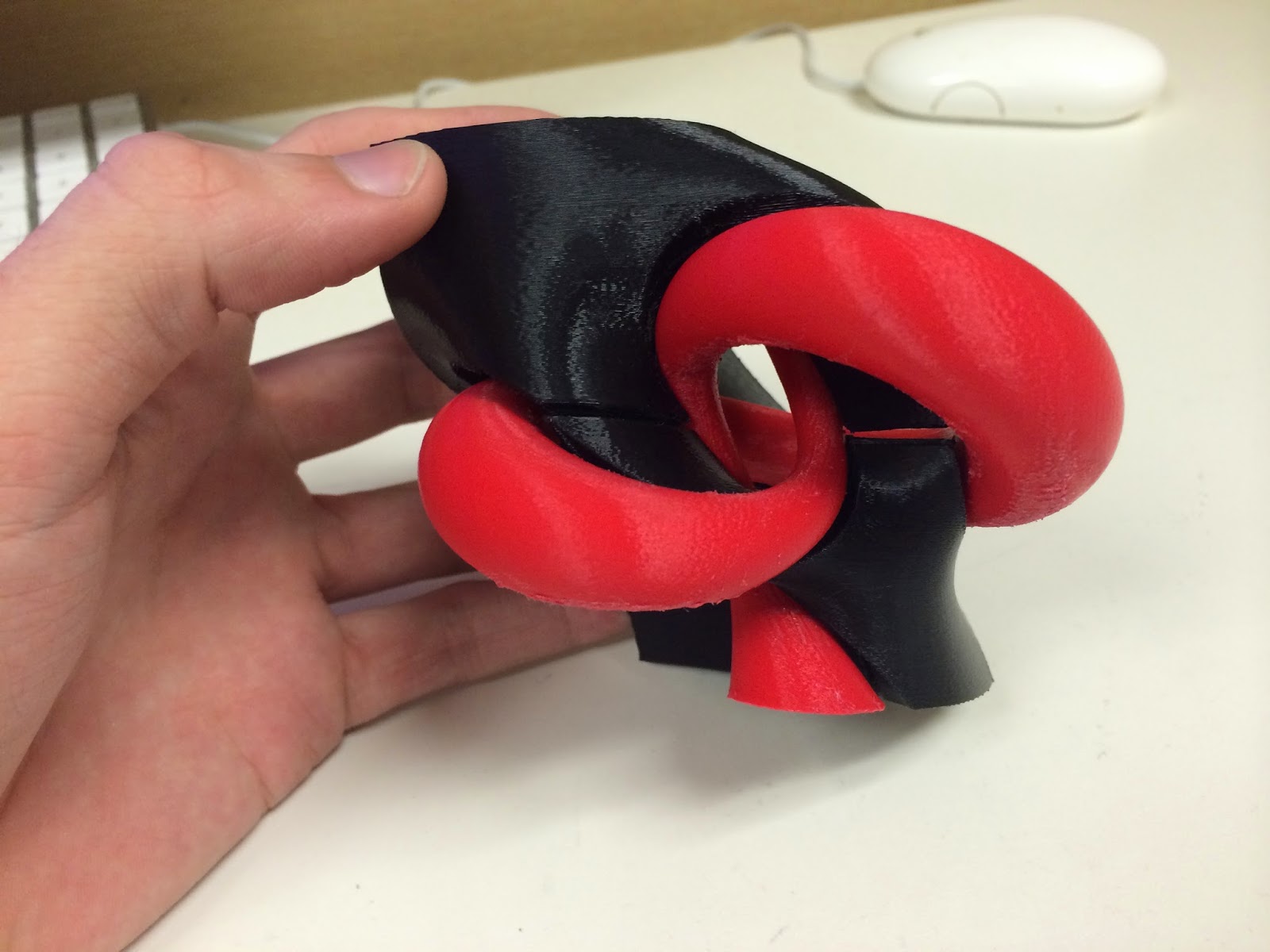
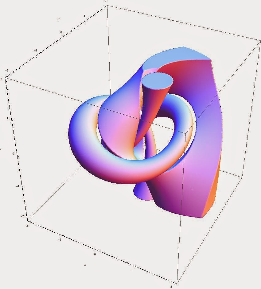
The goal of this project is to create a 3D puzzle of the trefoil knot and its fibrations via 3D printing. This is a long post but here is what we we will build at the end of this project:

Let’s start with some theory.

Theory and Stereographic Projection

Consider the following function from $\mathbb{C}^2$ to $\mathbb{C}$ (we can think of this as a function from $\mathbb{R}^4$ to $\mathbb{R}^2$ - see the Wikipedia entries for real n-space and complex n-space for more information): this function sends a coordinate pair $(u, v)$, where $u$ and $v$ are complex numbers, to the quantity $(u+i v)^2 - (u-i v)^3$, where $i = \sqrt{-1}$. This particular function’s zero-set, a set of points $(u,v)$ such that $(u+i v)^2=(u-i v)^3$, generates a trefoil knot through infinity. By considering inverse images of certain subsets of $\mathbb{C}$ we will generate a trefoil knot given our function’s zero-set; however, this inverse image is a subset of $\mathbb{C}^2$. To obtain our knot and understand its subsets better, we need a method to realize our object in $\mathbb{R}^3$.

As a preliminary example, consider a sphere in $\mathbb{R}^3$ sitting on a plane (think of a ball sitting on a table). From the top of the sphere (think North Pole), draw a line segment downward through the sphere and ending at the table. Notice that this line segment intersects both the sphere and table once. We can do this same line drawing method over and over to obtain a one-to-one correlation from the sphere to the plane, i.e., every point (well, minus the exact top of the sphere!) on the sphere can be mapped to the plane. This is called stereographic projection, and Henry Segerman (henryseg on Thingiverse) has created a fantastic 3D printed model illustrating this method:

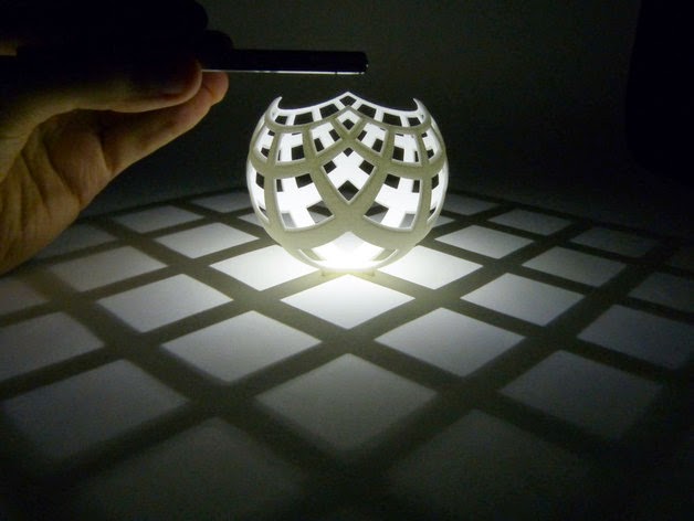
If we have a point light source (smartphone camera flash) and place it at the top of this model, light rays will act as the line segments in the above example. If held at the correct height, we should see the Cartesian grid on the table. I always keep this model in my backpack to demonstrate to people stereographic projection—I recommend printing it out!

So stereographic projection is a function from the unit sphere in $\mathbb{R}^3$ onto $\mathbb{R}^2$, but recall that our function is defined in $\mathbb{R}^4$. For us to embed our object in $\mathbb{R}^3$, we use a generalized version of stereographic projection to go from the unit sphere in $\mathbb{R}^4$ to $\mathbb{R}^3$. With this tool, we can compose the inverse stereographic projection function with our function defined above. So our new function now goes from $\mathbb{R}^3 \rightarrow \mathbb{C}$.

If we take inverse images of subsets of $\mathbb{C}$, we now have a function that goes from $\mathbb{C} \rightarrow \mathbb{C}^2 = \mathbb{R}^4 \rightarrow \mathbb{R}^3$, i.e., our single, final function takes in certain subsets of $\mathbb{C}$ and outputs subsets of $\mathbb{R}^3$—exactly what we want!

Mathematica, Plotting, and Resolution

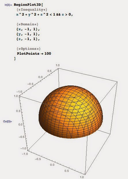
To generate 3D computer models of the trefoil knots, I chose to use Mathematica. RegionPlot3D, a built-in Mathematica function, plots regions in 3D space using inequalities. In order to use RegionPlot3D, the user must specify the domain of values to plot over in the $x$, $y$, and $z$ directions, as well as a mathematical inequality. As an example we can generate a sphere of radius 1 by the following code:

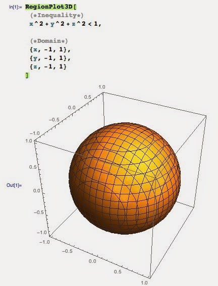
Mathematica will plot all points $(x, y, z)$ such that each point falls within the considered domain and obeys the given inequalities—but we can take this further. We can use multiple inequalities using boolean operators such as AND and OR. As an example, let’s consider the same sphere defined above, but restrict the region so that only points above the plane $z=0$ are plotted.

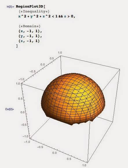
Of course we could restrict the $z$ range so that $z$ goes from $(0, 1)$, but it is nice to be able to manipulate a model without changing the overall plotted region. When models become more complicated this method allows us to control individual components without altering other pieces.

Before we start creating trefoil knots, there is one last Mathematica option that needs to be discussed: PlotPoints. Notice how choppy and non-circular the bottom of our hemisphere looks in the image above—PlotPoints will fix this. The PlotPoints function can be thought of as the resolution of a 3D model. A higher PlotPoints value tells Mathematica to use more points to represent the plotted region. However, as we increase PlotPoints, we also increase computation time. Say we used a PlotPoints of 50 and the model was under-represented. We could double our resolution and set PlotPoints to 100, but remember we are in 3D space, so by doubling the number of points in all directions $x$, $y$, and $z$ we increase our computation by $2\times2\times2=8$. In other words, doubling a model’s resolution increases computation time by a factor of 8. So let’s plot that same hemisphere with a PlotPoints of 100 and see what the bottom looks like.

Much better! Now that we have an understanding of RegionPlot3D and PlotPoints, it’s time to create some trefoil knots.

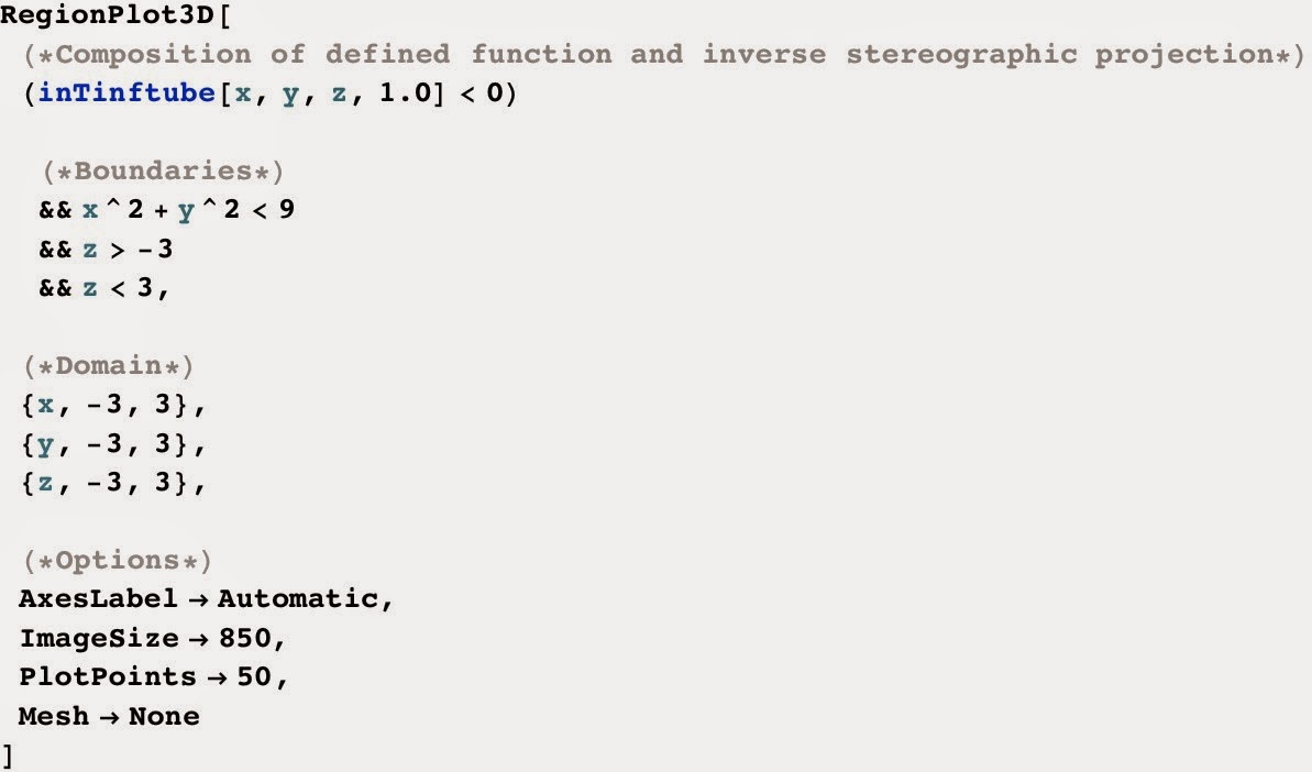
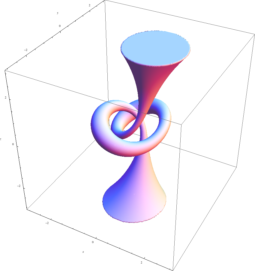
The main Mathematica function I wrote, inTinftube, defines the trefoil knot (the composition of our trefoil knot function with inverse stereographic projection explained above) by inputting points $(x, y, z)$ and “knot thickness” and returning a single number. Inside the function it tests points using inequalities such that if the outputted number is less than 0, Mathematica includes the point in the plot, and if the number is greater than 0, Mathematica does not include the point in the plot. We also need to define a boundary condition, otherwise our model would stretch to infinity! So we can include more inequalities that points must satisfy such that our boundary is a cylinder of radius 3, height 6, and is centered at the origin. With these parameters selected, the results below depict our “standard” trefoil knot. This knot is the inverse image of a small disk around 0 in $\mathbb{C}$ to give the knot thickness—a visual description of this will be shown in the next section.

Thingiverse link: http://www.thingiverse.com/thing:243260

Open Book Decomposition, Fibrations, and Pages.

Now that we have our “standard/reference trefoil knot,” it is time to start adding fibrations. To do this, unravel the above trefoil so that it is a straight strand. Consider that cord the spine of a book. Now add in one page to the book; the page will connect to the spine along one edge. Now twist the cord back into the trefoil knot configuration—what does the page, i.e., knot fibration, look like? This idea is called an Open Book Decomposition.

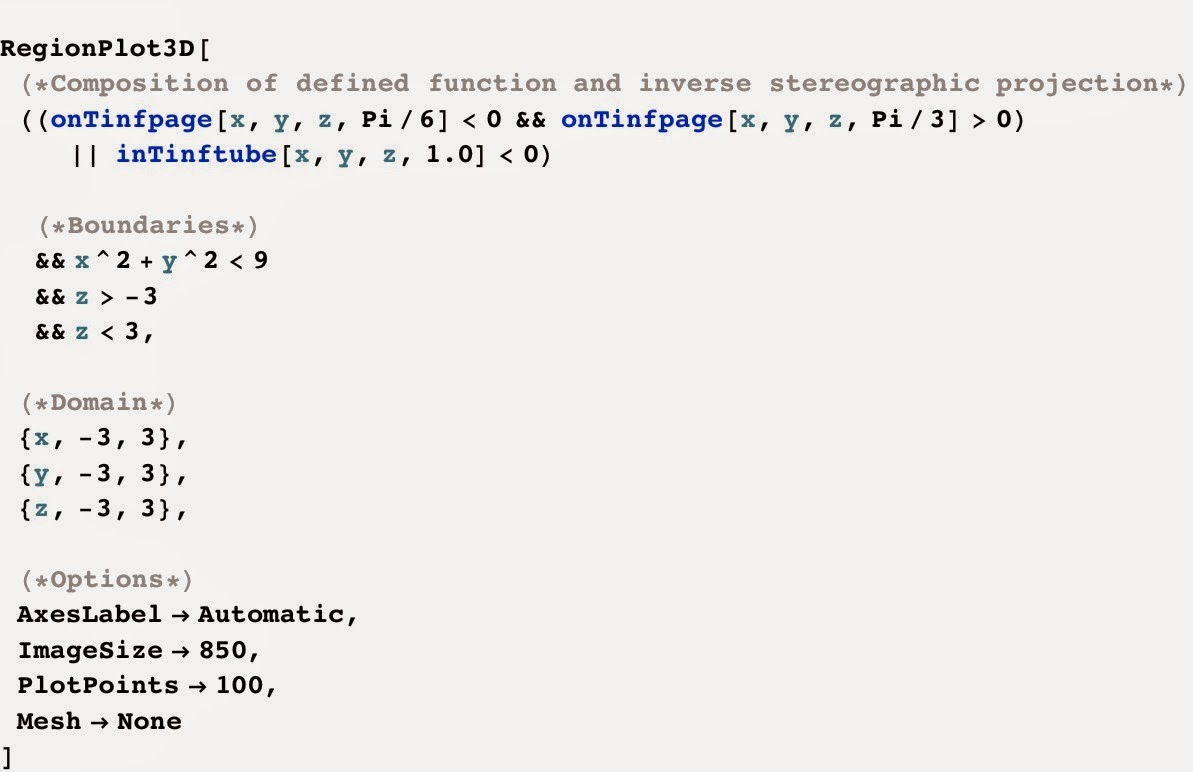
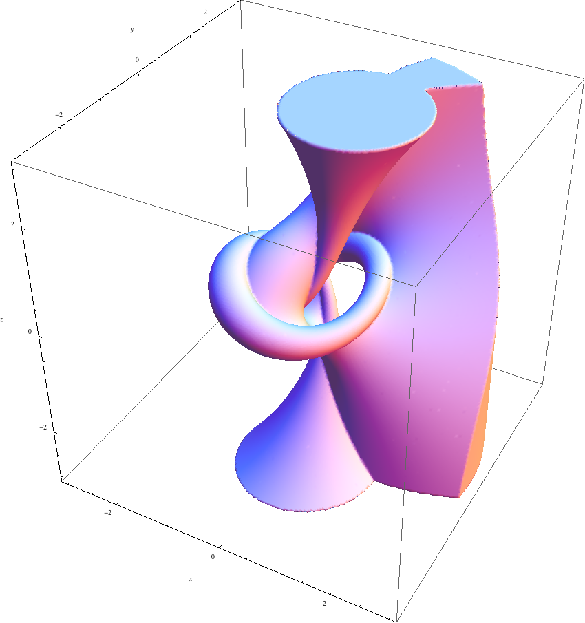
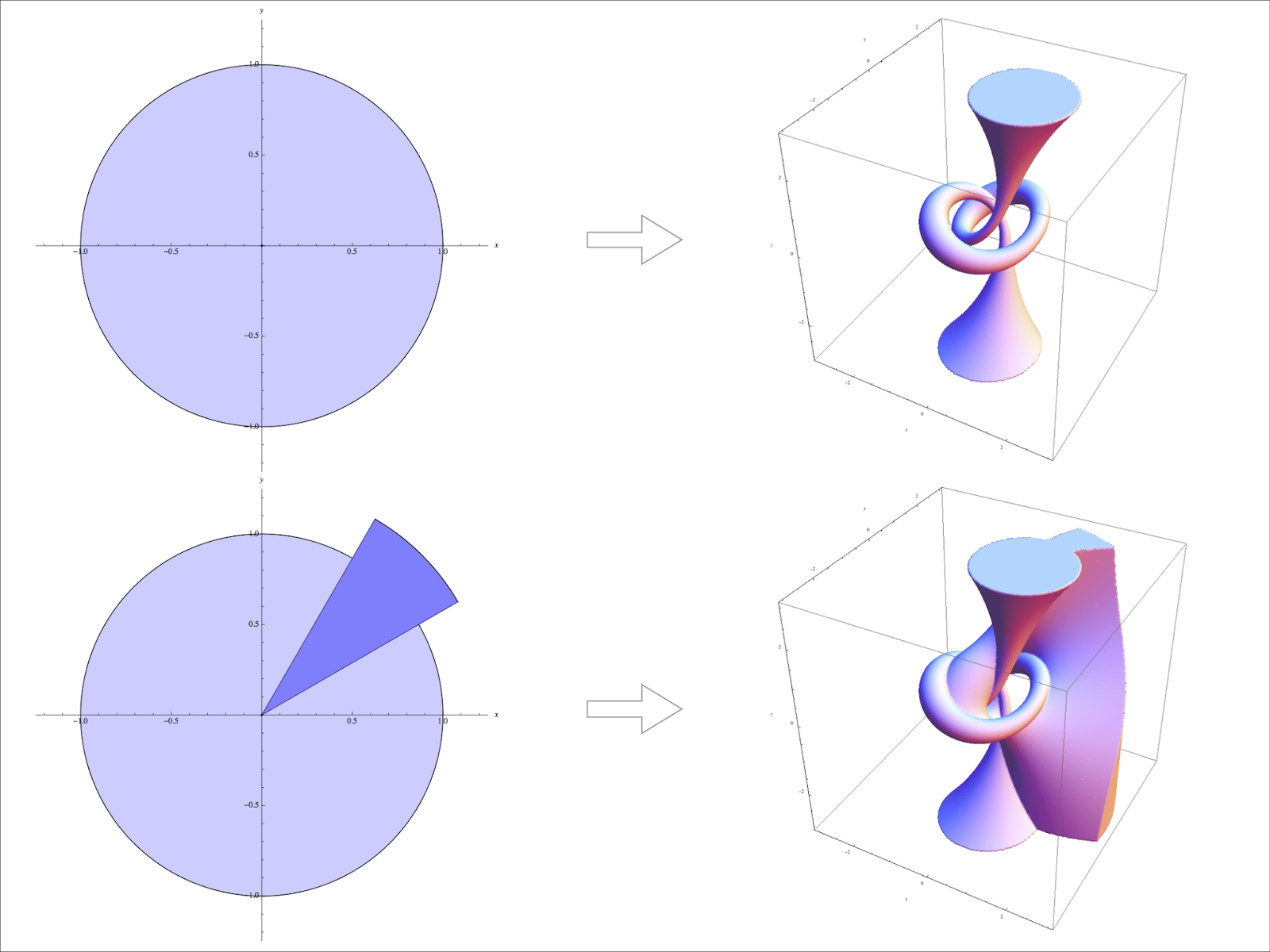
We can visualize this by adding extra regions to the model in $\mathbb{C}$ before we apply our single function. To do this, I wrote another Mathematica function, inTinfpage, that takes in points and outputs a number; however, this time the function also requires an angle. This angle will define a ray in the plane starting at the origin that is rotated an angle in the mathematically positive direction. As before, we can have Mathematica plot points if the outputted number is below zero, but we want a page of some physical thickness (in order to 3D print). For most of my successful prints I have been using a page thickness of $\pi/6$. So we can now include another “ray-function” and input an angle that is $\pi/6$ larger than before and have Mathematica plot things that are greater than 0. We have now included another region in the plane. This process is much easier to see in the image below.

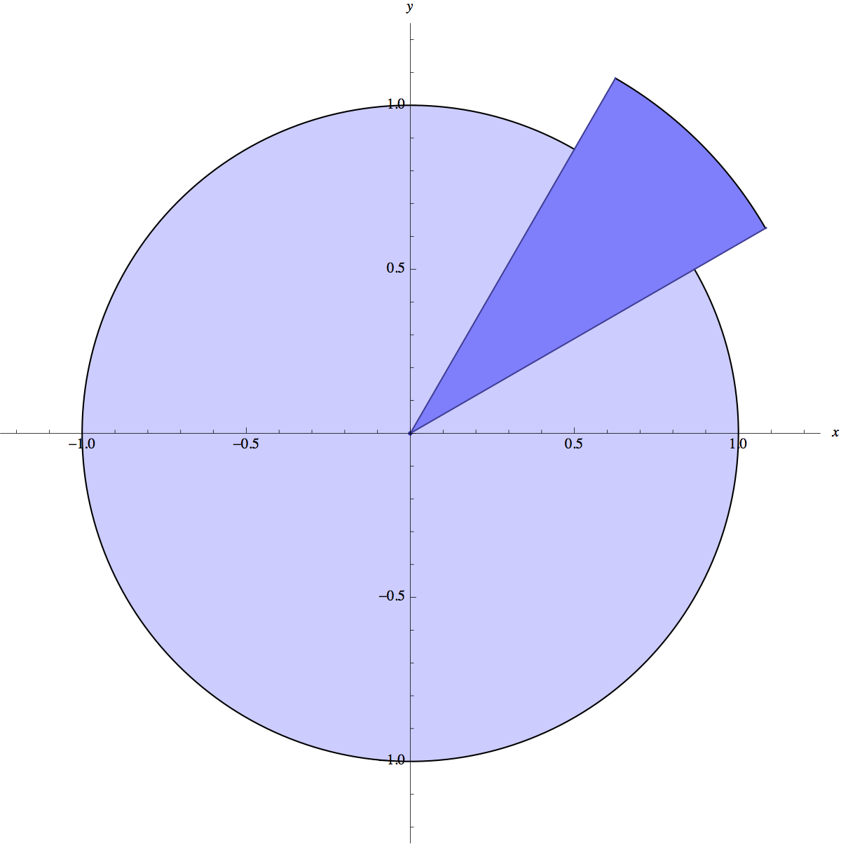
The circle is the radius of the trefoil knot, and the region in the first quadrant is our fiber with thickness. That’s the new region we want to include when using stereographic projection. Remember the picture above is the subset of $\mathbb{C}$ that we are taking inverse images of. We can now apply our same code to generate the following model.

Why stop at one extra region? We can add as many as we would like, and at $\pi/6$ thickness, we should be able to fit 12 extra regions in our trefoil knot (since $\pi/6\times12=2\pi$). Some other examples are below, with the region in $\mathbb{C}$ shown on the left, and its inverse image (after applying stereographic projection) shown on the right.

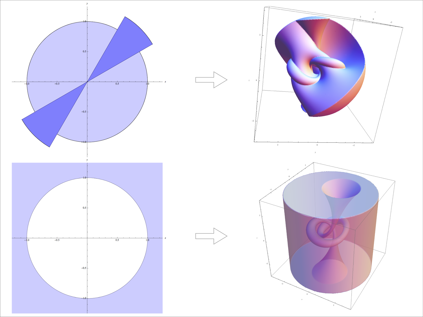
We can now start to see the consequences of projecting our 4D function into $\mathbb{R}^3$, which is why our knots are visually unlike typical trefoil knots.

Now that I have code that can generate trefoil knots and fibrations of any thickness, it’s time to start printing various versions of the models. The goal is to be able to print the trefoil knot separate from the pages to create a 3D puzzle. At the end of this post I’ll share some of my successful experiments in doing just that.

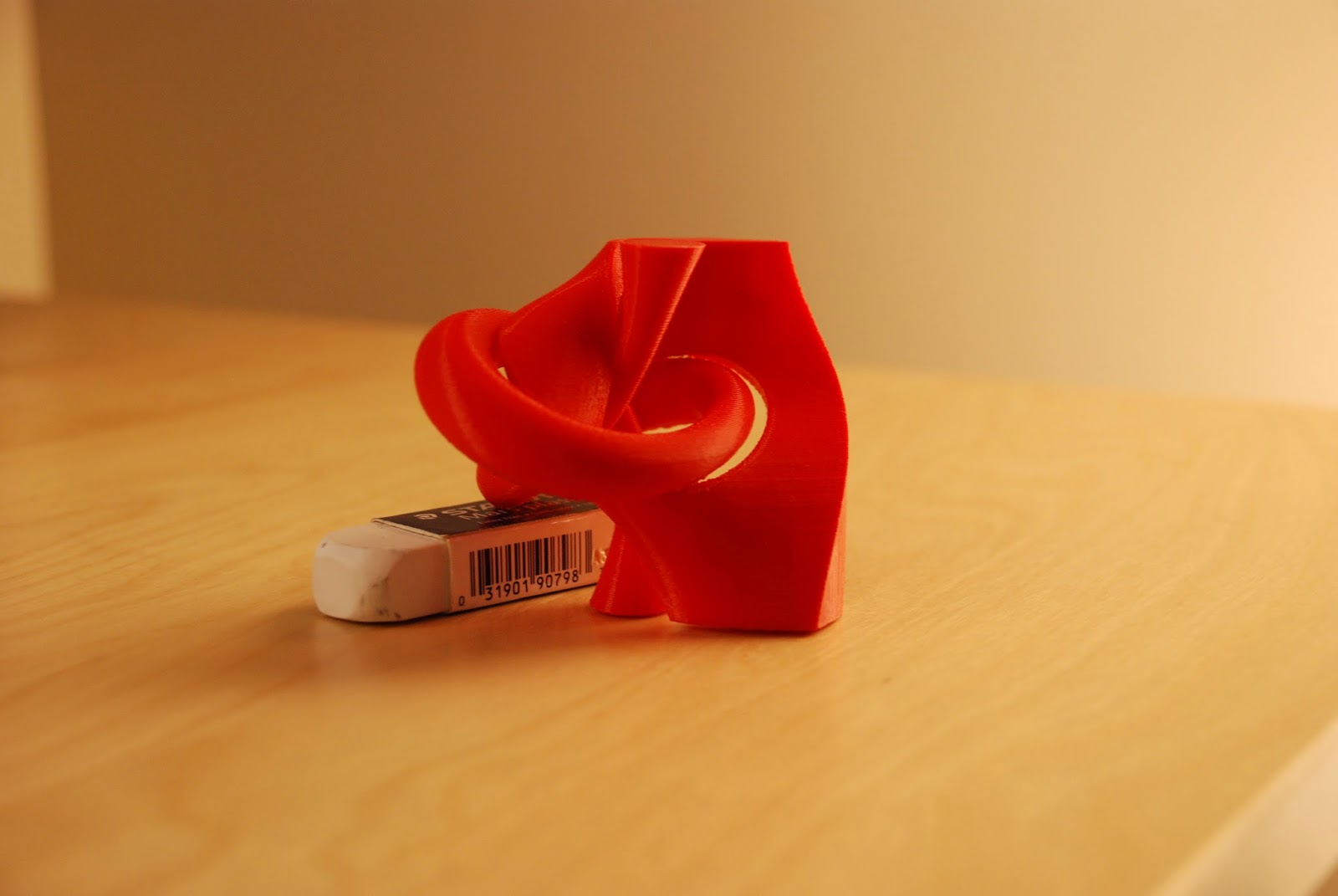
1. Printing the trefoil knot with one page with a gap.

Here I made a model of the trefoil knot with one page, but removed the points where the page meets the knot. In other words, there is a gap running along the knot where the page meets the surface of the knot. When printed, the page should be free to wiggle a little bit. Here is the object in Mathematica:

After exporting to STL and printing, this is the result:

Thingiverse link: http://www.thingiverse.com/thing:331530

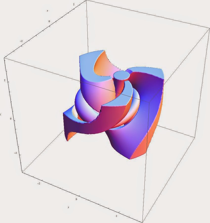
2. Printing the trefoil knot with three pages with a gap.

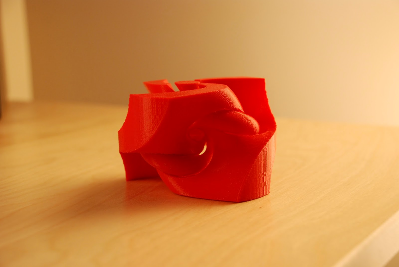
This is a trefoil knot with three pages, all of which have gaps where the pages meet the knot. This knot is closely related to the previous model; however, two more pages have been added, all of which are equiangular (think of the Mercedes Benz logo). The print time on this can be a bit longer (an afternoon), and the clean-up of supports can get annoying. However, this model looks fantastic in person. Here it is in Mathematica:

And now printed:

Thingiverse link: http://www.thingiverse.com/thing:337185

3. Printing the trefoil knot and one page separately.

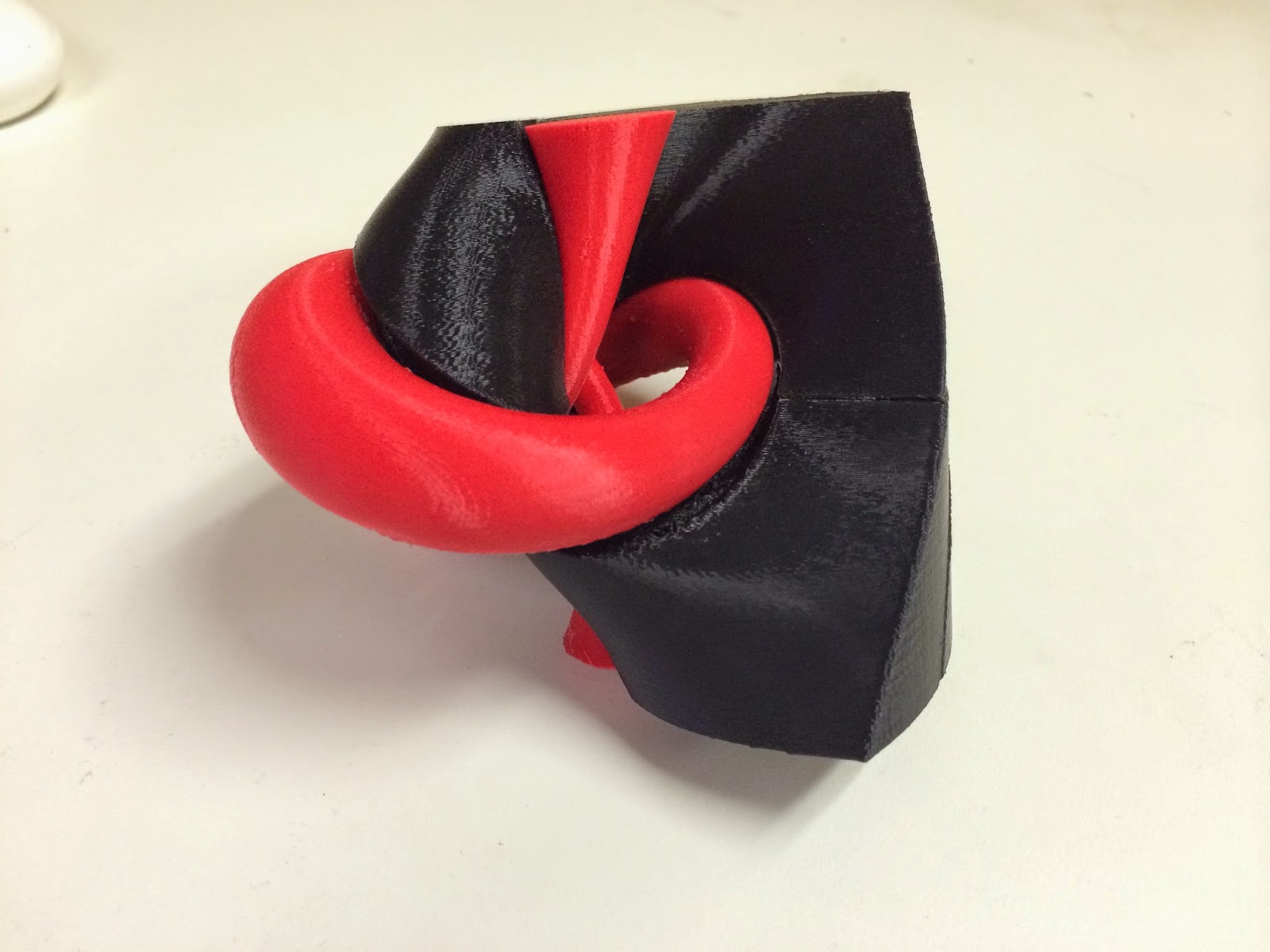
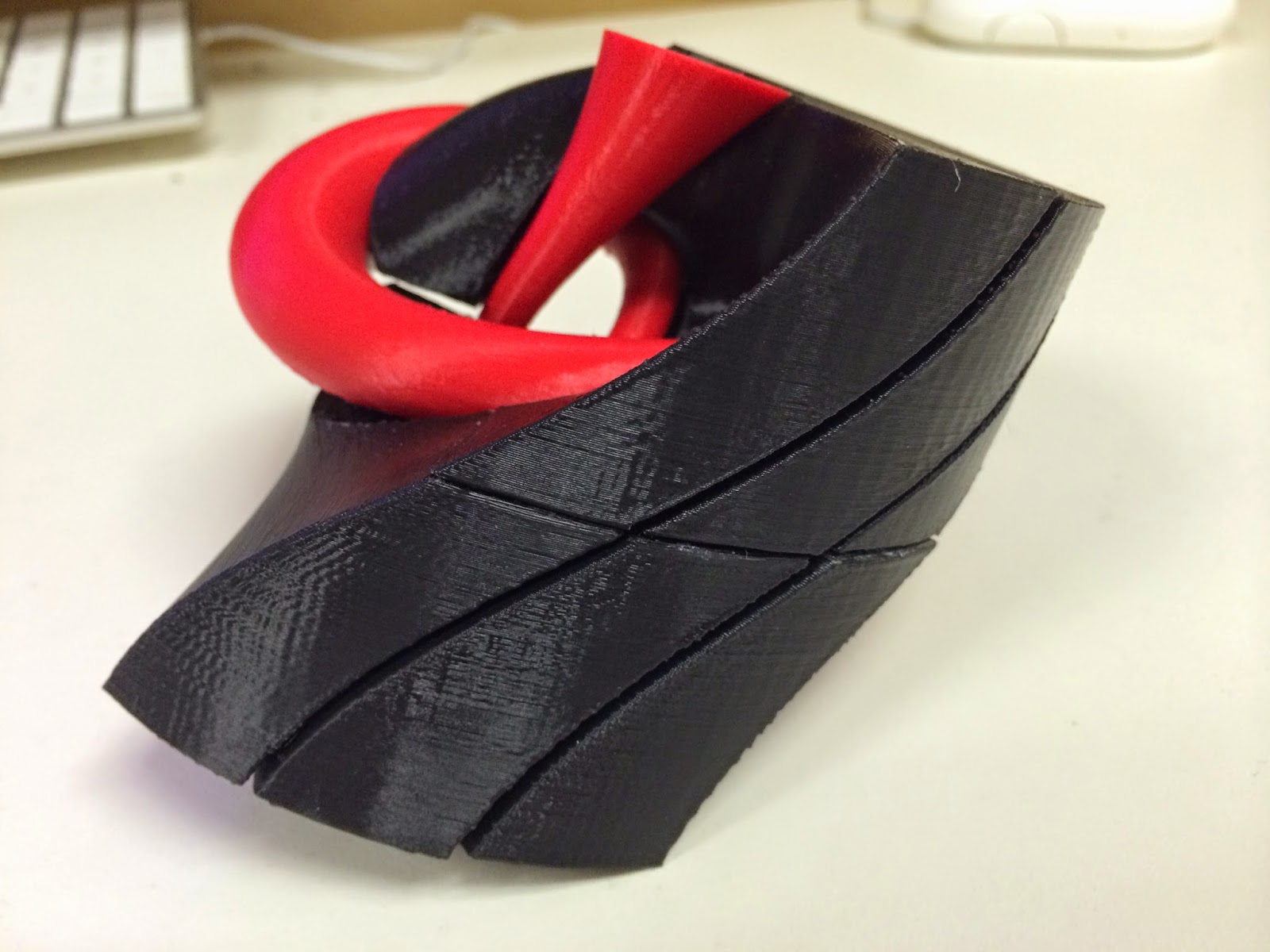
Here I printed the standard trefoil knot but edited the domain so that the knot itself is bigger. I also made a groove in the knot that follows where one page meets the surface, with hopes that if I could print a page separately, then I could snap the page into the knot. Next, I took one page and split it into two pieces with the plane $z=0$. With a little force, I was able to get both pieces in the knot. A good first start, but not ideal for consistent “puzzle-building”.

Current and future work

This puzzle-building problem illustrates a simple idea, but can prove to be very complicated in practice. Many people have assembled large objects by printing smaller components; however, due to the complex geometry of the shape we are dealing with, slicing the knot in a particular way such that the pieces can be reassembled without blocking any other piece is an interesting and challenging problem for any 3D printing enthusiast.

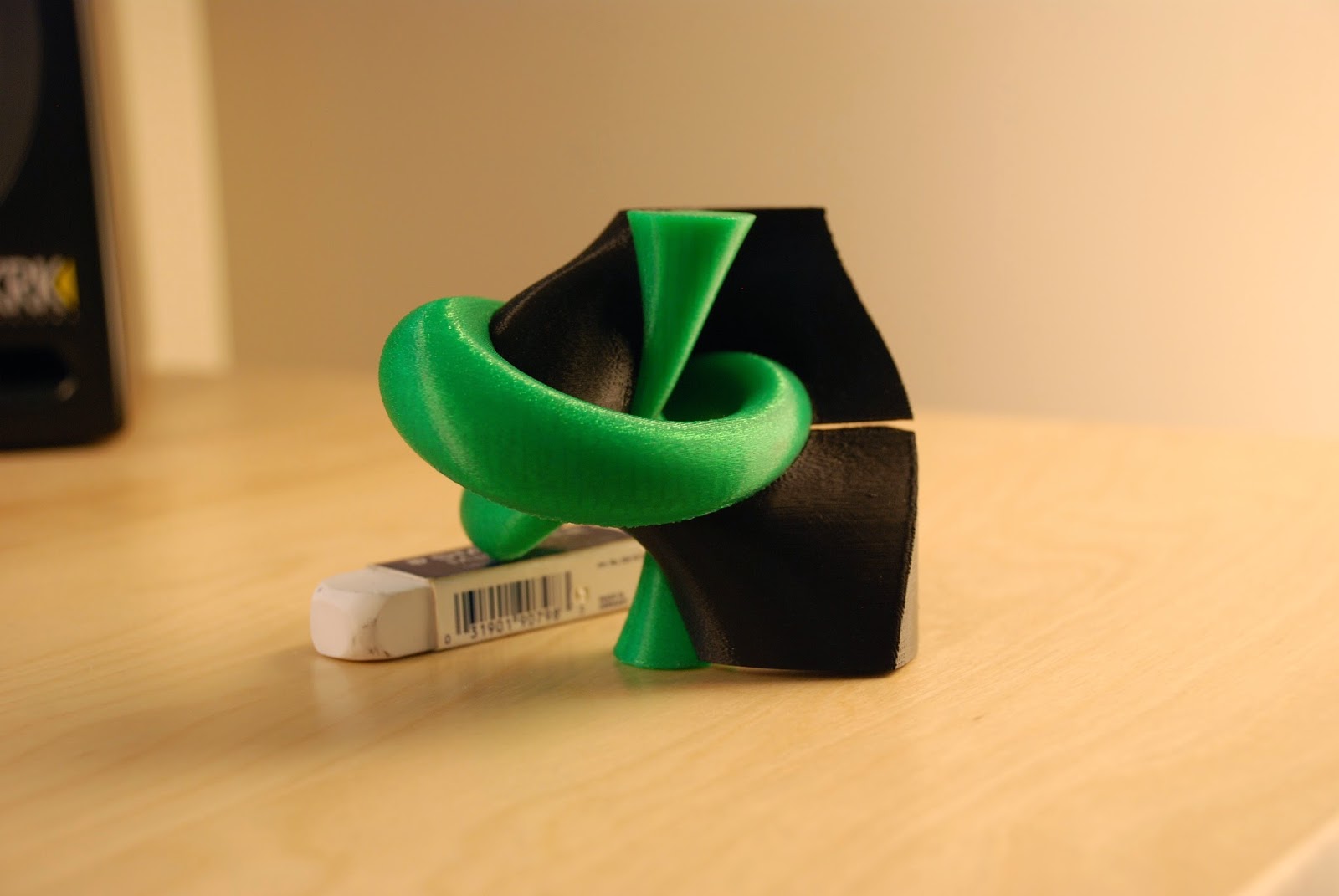
My latest attempt has been to have Mathematica generate all twelve pages of $\pi/6$ thickness, cut each page into two pieces using the plane $z=0$, and import each piece individually into Blender, a free, open-source 3D modeling and animation software. In Blender, I added small holes in the bottom and top of each piece of a page. Once the hole was made, I printed the pieces of the pages and glued in small magnets to hold two pieces of the same page together (not all pages are same; in fact, every page is different from one another). I successfully printed a trefoil knot and 3 pages (6 pieces), all with magnets, to make a 7-piece 3D puzzle. Here is the process in Blender:

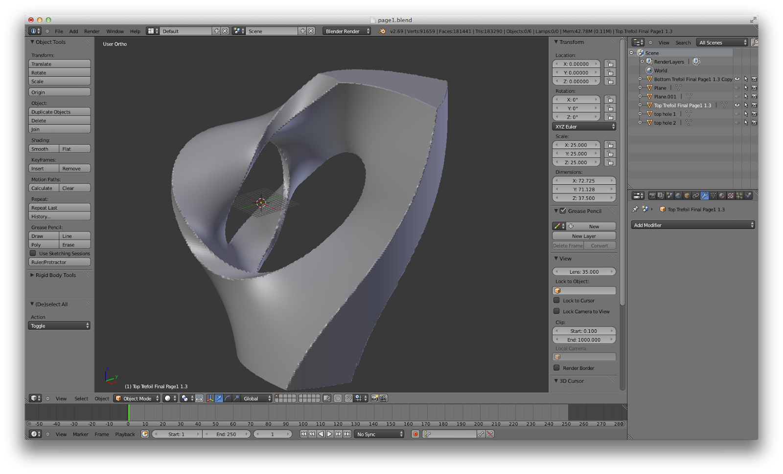
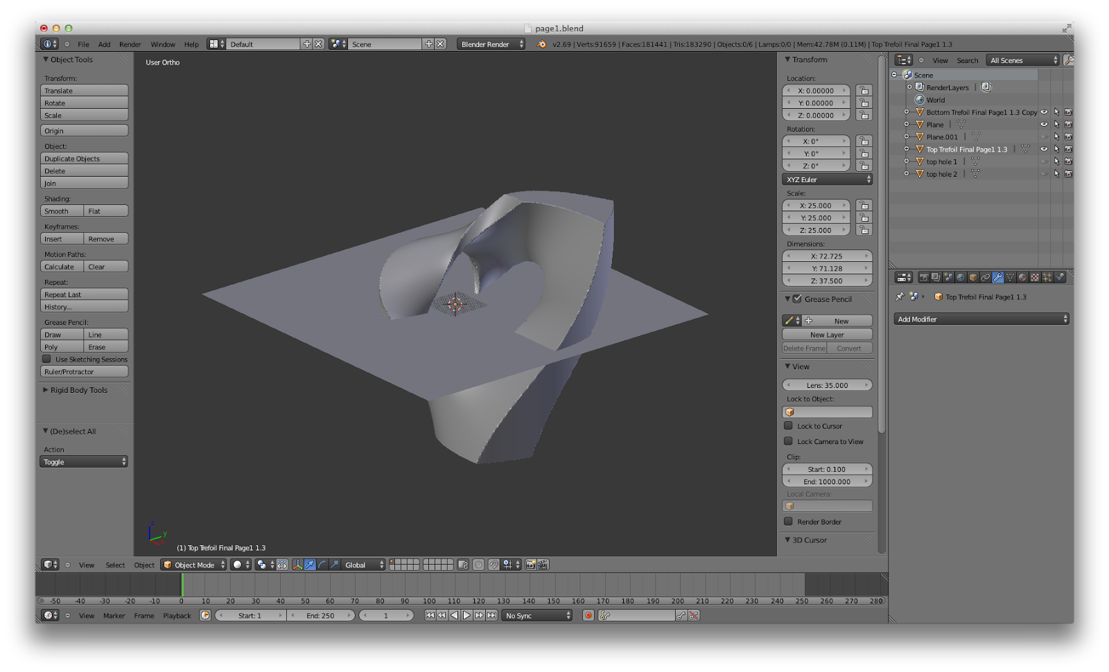
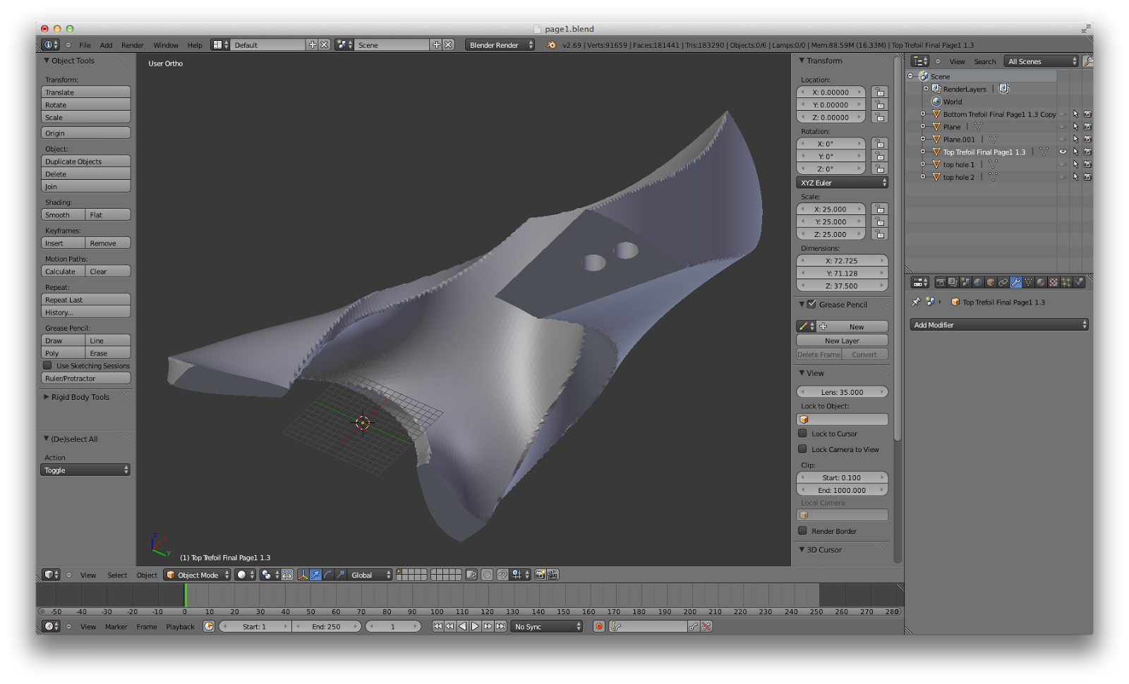
And here are the prints:

This coming year I will work to refine the process of adding holes; I may cut the pages at different angles too. Once a puzzle has been made and printed that is easy to piece together, contains multiple pieces, and is of appropriate size, I plan on posting the puzzle in its entirety on my Thingiverse profile — so be on the lookout!

I would like to thank Dr. Laura Taalman for the opportunity to write about my research so far, and Dr. David Gay at the University of Georgia for his guidance and access to a MakerBot Replicator 2.