Thank you very much! First one gets
In[3]:= NDSolve[{D[x^2 D[y[x], x], x] == -x^2 (y[x])^(3/2), y'[0] == 0, y[1] == 0}, y , {x, 0, 1},
 Method -> {"EquationSimplification" -> "Residual"}]

During evaluation of In[3]:= NDSolve::bvdae: Differential-algebraic equations must be given as initial value problems. >>

Out[3]= NDSolve[{2 x Derivative[1][y][x] + x^2 (y^\[Prime]\[Prime])[x] == -x^2 y[x]^(3/2),
  Derivative[1][y][0] == 0, y[1] == 0}, y, {x, 0, 1},
 Method -> {"EquationSimplification" -> "Residual"}]
but the initial problem can be used to shoot the boundary condition rather straightforward
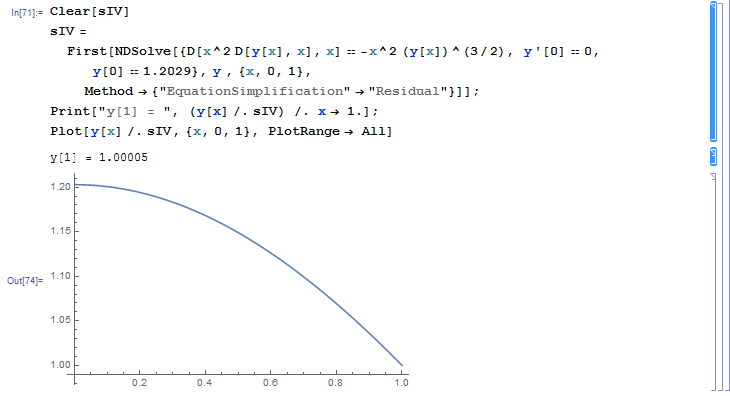
Clear[sIV]
sIV = First[NDSolve[{D[x^2 D[y[x], x], x] == -x^2 (y[x])^(3/2), y'[0] == 0, y[0] == 1.2029}, y , {x, 0, 1},
    Method -> {"EquationSimplification" -> "Residual"}]];
Print["y[1] = ", (y[x] /. sIV) /. x -> 1.];
Plot[y[x] /. sIV, {x, 0, 1}, PlotRange -> All]

y[1] = 1.00005
the plot is only interesting for the real p.o., but nevertheless here it is
