Message Boards Message Boards

0
|
9235 Views
|
3 Replies
|
5 Total Likes
View groups...
Share
Share this post:

SolveDelayed has died?

Posted 10 years ago

The referece still says (Mathematica 10.0.2 Win 7 64 Bit Home Premium)

?SolveDelayed

SolveDelayed is an option to NDSolve. SolveDelayed -> False causes the derivatives to be solved for symbolically at the beginning. SolveDelayed -> True causes the ODEs to be evaluated numerically and the derivatives solved for at each step.

let's use it

In[86]:= NDSolve[{2 x y'[x] + x^2 y''[x] + x^2 y[x] == 0, y'[0] == 0, 
  y[1] == 0}, y, {x, 0, 1}, Method -> {"Shooting"}, SolveDelayed -> True]

During evaluation of In[86]:= NDSolve::bvdae: Differential-algebraic equations must be given as initial value problems. >>

Out[86]= NDSolve[{x^2 y[x] + 2 x Derivative[1][y][x] + 
    x^2 (y^\[Prime]\[Prime])[x] == 0, Derivative[1][y][0] == 0, 
  y[1] == 0}, y, {x, 0, 1}, Method -> {"Shooting"}, 
 SolveDelayed -> True]

it's a linear ordinatry differential equation, what does the NDSolve::bvdae mean here? Does is mean SolveDelayed has died in NDSolve?

If the SolveDelayed is not specified, the NDSolve::bvdae does not show up and a numerical solution is generated.

POSTED BY: Udo Krause
3 Replies

This example from M. Trott, The Mathematica GuideBook for Numerics, ยง 1.11, (2006), p. 399 still works

SolveDelayed

so it seems at least partially a cosmetic problem (SolveDelayed in red).

POSTED BY: Udo Krause

SolveDelayed has been deprecated (it will continue working as before for backward compatibility). To treat the system as a DAE, instead of SolveDelayed -> True, one should use Method -> {"EquationSimplification" -> "Residual"}. See also the documentation. However, if this option is set, then the NDSolve::bdae message is expected, since there is no DAE support for boundary value problems.

POSTED BY: Ilian Gachevski

Thank you very much! First one gets

In[3]:= NDSolve[{D[x^2 D[y[x], x], x] == -x^2 (y[x])^(3/2), y'[0] == 0, y[1] == 0}, y , {x, 0, 1}, 
 Method -> {"EquationSimplification" -> "Residual"}]

During evaluation of In[3]:= NDSolve::bvdae: Differential-algebraic equations must be given as initial value problems. >>

Out[3]= NDSolve[{2 x Derivative[1][y][x] + x^2 (y^\[Prime]\[Prime])[x] == -x^2 y[x]^(3/2), 
  Derivative[1][y][0] == 0, y[1] == 0}, y, {x, 0, 1}, 
 Method -> {"EquationSimplification" -> "Residual"}]

but the initial problem can be used to shoot the boundary condition rather straightforward
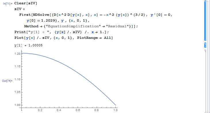
Clear[sIV]
sIV = First[NDSolve[{D[x^2 D[y[x], x], x] == -x^2 (y[x])^(3/2), y'[0] == 0, y[0] == 1.2029}, y , {x, 0, 1}, 
    Method -> {"EquationSimplification" -> "Residual"}]];
Print["y[1] = ", (y[x] /. sIV) /. x -> 1.];
Plot[y[x] /. sIV, {x, 0, 1}, PlotRange -> All]

y[1] = 1.00005

the plot is only interesting for the real p.o., but nevertheless here it is

dolhaineODE

POSTED BY: Udo Krause
Reply to this discussion
Community posts can be styled and formatted using the Markdown syntax.
Reply Preview
Attachments
Remove
or Discard

Group Abstract Group Abstract