Hello Benjamin,

It would be better if you posted your code by putting it in a separate paragraph, selecting it and using the Code Sample button on the far left above the panel.

There are some syntax errors in your expression. You should not use double brackets on the Cos[[CurlyPhi]] expression and you enter the CurlyPhi by using esc j esc. So that part of the expression should be entered as Cos[esc j esc]. The you might define your function this way:

f[x_, \[CurlyPhi]_] = 
 3.36429*10^-9 (-1500 + x) + 
  0.012242 E^(-0.0428469 x) Cos[
    0.0428469 x] (0.000818033 + 
     0.308311 Cos[\[CurlyPhi]]) + (-0.844704 Cos[\[CurlyPhi]] - 
     1.40784*10^-6 (-1500 + x)^2 Cos[\[CurlyPhi]])/2100 - 
  0.000524531 E^(-0.0428469 x) (0.00947115 + 
     3.55308 Cos[\[CurlyPhi]]) (Cos[0.0428469 x] - Sin[0.0428469 x])

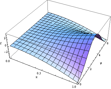
Here I scale the function up by 10^6 just to have better coordinates on the plot.

One possible plot is:

Plot3D[10^6 f[x, \[CurlyPhi]], {x, 0, 1}, {\[CurlyPhi], 0, 2 \[Pi]},
 AxesLabel -> {"x", "\[CurlyPhi]", "f"}]

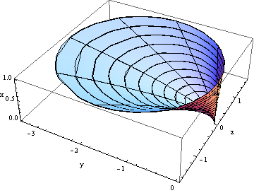
Another possible plot is:

RevolutionPlot3D[{10^6 f[x, \[CurlyPhi]], x}, {x, 0, 1}, {\[CurlyPhi],
   0, 2 \[Pi]},
 AxesLabel -> {"y", "z", "x"}]