plz someone help me in this regard I have uploaded the file ,I have tried my level best but unable to find error.

For Contour plot , whynot you consider the range of mu, mu-3sigma to mu + 3 sigma, why you do this only for lambda.

Okay .. but what about simulation if I want to simmulate the above code ??

jim Thanx a lot, its really a great help from your side. Once again a big thanx. As for as your question is concerned , Yes I m interested in mixture distribution. But firstly I do it for simple case , Now sir my question regarding to above programme are (1): its only for one data set .I need for repeated times like 1000 , or 10,000 times that we get 10000 mle and variance covariance matrices and on the average we report the results. (2): Second is will you plz explain the contour plot I mean its command and its interpretation . Third and last question is there is iterative method like newton raphson method how that can be used for mle and variance covariance .

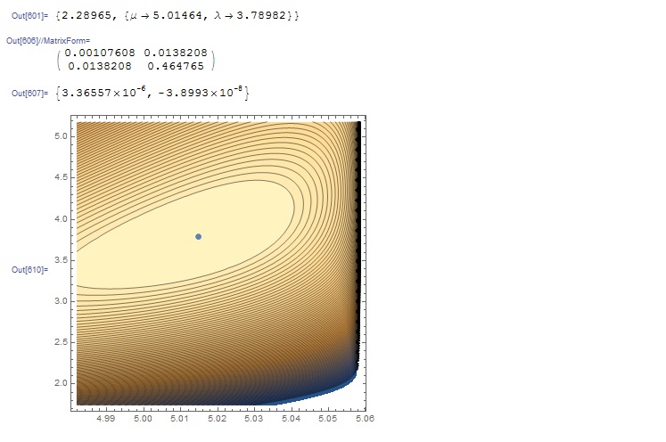
I made a few corrections. (One correction is the need to have separate variables for the parameters to generate the data and the parameters to be estimated.) For this log likelihood, Maximize works better than NSolve (in part I think because maximum likelihood estimator of mu is so close to the minimum data value). I also added some QA checks to see if the solution makes sense (which for just about any iterative method is highly recommended).

The estimate of the covariance matrix is also included but I wonder if because you are doing simulations and looking to characterize the sampling distributions of the maximum likelihood estimates, do you really need that? The "true" covariance matrix would be estimated from the results of the multiple simulations performed (unless you're also interested in the sampling properties of the estimated covariance matrix).

Below is the code:

(*Maximum likelihood example*)

(*Set parameter values*)
n = 50; \[Mu]0 = 5; \[Lambda]0 = 3;

(* Generate data *)
u = RandomReal[UniformDistribution[{0, 1}], n];
x = \[Mu]0 + Sqrt[Log[1 - u]/-\[Lambda]0];

(* Log likelihood *)
logL = n*Log[2] + n*Log[\[Lambda]] + \!\(
\*UnderoverscriptBox[\(\[Sum]\), \(i = 1\), \(n\)]\(Log[
     x[\([i]\)] - \[Mu]]\)\) - \[Lambda]*\!\(
\*UnderoverscriptBox[\(\[Sum]\), \(i = 1\), \(n\)]
\*SuperscriptBox[\((x[\([i]\)] - \[Mu])\), \(2\)]\);

(* Find maximum likelihood estimates *)
sol = Maximize[{logL, \[Mu] < Min[x] && \[Lambda] > 
     0}, {\[Mu], \[Lambda]}]
mle = {\[Mu], \[Lambda]} /. sol[[2]];

(* First order partials *)
DlogL = D[logL, {{\[Mu], \[Lambda]}}];

(* Calculate variance estimates using second order partials *)
hessian = D[DlogL, {{\[Mu], \[Lambda]}}] /. sol[[2]];
v = -Inverse[hessian];
MatrixForm[v]

(* Check to see that the first order partials are close to zero with \
estimates of \[Mu] and \[Lambda] *)
DlogL /. sol[[2]]

(* Additional check:  show contour plot of log likelihood around the \
mle's *)
c = ContourPlot[logL, {\[Mu], mle[[1]] - v[[1, 1]]^0.5, Min[x]},
   {\[Lambda], mle[[2]] - 3 v[[2, 2]]^0.5, mle[[2]] + 3 v[[2, 2]]}, 
   Contours -> 100];
m = ListPlot[{mle}];
Show[{c, m}]

with the following output:

This community will work fine for any discussions (although the discussion has been a bit one-sided so far - but that can change).

Jim can you plz give me your mailing Id ?? I need to discuss plz do me a favour.

You know for likelihood estimates we differentiate log- likelihood function with respect to paramerters , as a result we get some implicite or explicit form of equations with respect to parameters , I need their variance covariance matrix also

I (always) highly recommend the book by Rose and Smith: Mathematical Statistics with Mathematica. There's a great chapter on symbolic maximum likelihood estimation. (Although maybe your mention of "simulations" might mean you would be more interested in numerical rather than symbolic solutions.)