Stress testing in the Value-of-Risk context provides complementary view of the firms risk profile when market becomes extremely volatile and unstable. In this respect, the stress testing generally replicates crisis scenarios in the current market setting. Traditional approach to stress testing emphasises qualitative factors. We propose alternative arrangement - purely quantitative approach with probabilistic setting where particular stress test is modelled thought the quantiles of the calibrated probability distribution.
Introduction
Value-at-Risk (VaR) as a standard risk measure is usually defined in terms of time horizon, confidence interval and parameters setting that drive the calculation of the measure. There are few theoretical underlying assumptions behind VaR and one f them refers to VaR as the measure under the normal market conditions. This fundamental principle, by definition, is meant to ignore extreme market scenarios where market parameters - and the volatility in particular - undergoes a period of excessive variations.
Stress testing plays a complementary function to VaR - it identifies the hidden vulnerability of the risk measure as a result of hidden assumptions and thus provides risk and senior managers with a clear view of the loss when market runs into crisis.Therefore, financial institutions these days are required to run the stress testing of their VaR on regular basis to quantify additional loss based on stress-affected para maters.
To ease and streamline the stress testing exercise we papoose new approach to stress testing based on probabilistic representation of VaR variables where particular scenario is modelled through the quantile behaviour of calibrated density. This approach is flexible, easy to implement and leads to elegant and tractable solution that can be applied in various risk quantification settings.
Stress definition
Stress testing is generally carried away in three settings:
- Historical scenario of particular crisis
- Stylised definition of particular scenarios
- Hypothetical events
The recent regulatory review strongly prefers the historical scenario approach where particular period with consecutive 12 months observation of crisis has to be included into the stress testing exercise.
The objective of this paper is to propose a new parametric approach to stress testing where the underlying market parameters are defined probabilistically and the stress scenario is then expressed as a quantile of certain probability distribution. The solution brings a number of benefits - the primary being simplicity of implementation, ease of maintenance and ease of use.
Problem setting
Consider the following case - we have built a portfolio of 5 UK stocks - Lloyds, Vodafone, Barclays, BP and HSBC - with £1 million invested in each of them. We want to compute VaR and stressed VaR for our portfolio with £5 million value.
Getting market data
We get the market data for the 5 stocks with a long history from Jan 2008
stocks = {"LLOY.L", "VOD.L", "BARC.L", "BP.L", "HSBA.L"};
data = TimeSeries[FinancialData[#, "January 1, 2008"]] & /@ stocks;
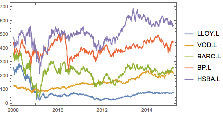
The price history of each stock looks as follows:
DateListPlot[data, PlotLegends -> stocks]
Processing market data
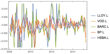
dret = TimeSeriesResample[MovingMap[Log[Last[#]] - Log[First[#]] &, data, {2}]];
In the same way we calculate each stock historical daily volatility
qvol = MovingMap[StandardDeviation, dret, {60, "Day"}];
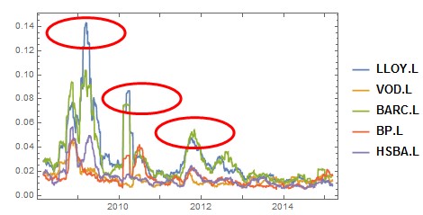
Evaluate@DateListPlot[qvol, PlotRange -> All, PlotLegends -> stocks]
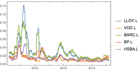
Both return and its volatility reveal high values for financial stocks - Lloyds and Barclays in particular- with excessive movement in 2009, 2010 and partially in 2012.
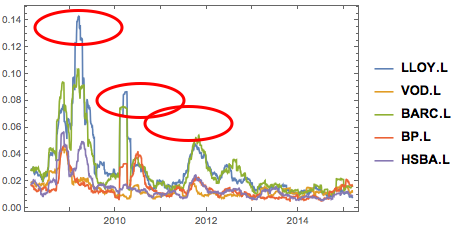
This are the periods that represent the peak of financial crisis and the stress to the market.
Probabilistic definition of volatility
VaR metrics is primarily dealing with the return volatility and therefore the volatility behaviour in the key object of the stress testing process. As the graph above suggests, the volatility evolution over time is not constant and we observe periods of high and low values. If we make an abstract view on the volatility data in general, we can treat it as a 'random variable' with some probability distribution. Presence of high and low values strongly supports this argument.
We propose Johnson distribution - unbounded type - to define the distribution of volatility density over the observed period of time. Let's recall that Johnson distributions represent a framework of distribution family in the from Y=[Sigma] g((X-[Gamma])/[Delta])+[Mu] where X~Normal[]. In case of 'unbounded' distribution the function g=sinh(x). The Johnson distribution family are well-behaved functions and with four parameters to use are therefore ideally suited for the data fitting with long and patchy tails. In this respect they can be easily used to model the volatility distribution over time.
The probability density of the Johnson unbounded distribution is:
PDF[JohnsonDistribution["SU", \[Gamma], \[Delta], \[Mu], \[Sigma]], x]
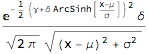
and the density plot with varying shape factor [Gamma] looks as follows:
Plot[Evaluate@
  Table[PDF[JohnsonDistribution["SU", \[Gamma], 1.25, 0.007, 0.00341],
     x], {\[Gamma], {-3, -4, -5}}], {x, 0, 0.15}, Filling -> Axis,
 PlotRange -> All,
 PlotLegends -> {"\[Gamma]=-3", "\[Gamma]=-4", "\[Gamma]=-5"}]
Johnson type of distributions are very flexible in terms of tail control.
Historical distribution of volatility
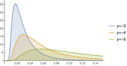
We can visualise the volatility distribution by looking at each stock histogram:
size = Length[stocks];
Table[Histogram[qvol[[i, All, 2]], 30, "PDF",
  PlotLabel -> stocks[[i]],
  ColorFunction ->
   Function[{height}, ColorData["Rainbow"][height]]], {i, size}]
We can use the historical data to fit the volatility to the Johnson distribution:
edist = Table[
  EstimatedDistribution[qvol[[i, All, 2]],
   JohnsonDistribution [
    "SU", \[Gamma], \[Delta], \[Mu], \[Sigma]]], {i, size}]
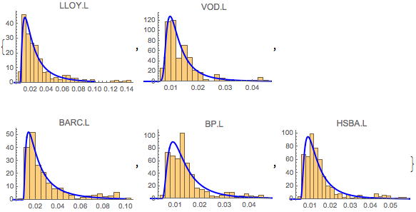
How good is the fit? We can observe this on the charts:
Table[Show[
  Histogram[qvol[[i, All, 2]], 20, "PDF", PlotLabel -> stocks[[i]]],
  Plot[PDF[edist[[i]], x], {x, 0, 0.1}, PlotRange -> All,
   PlotStyle -> {Blue, Thick}]], {i, size}]
Defining correlation matrix
Portfolio VaR requires correlation structure amongst the VaR components. We can create it from the historical return data defined above.The only problem is to define the time window from which we select the market data. For the standard VaR we can choose the one year history
tswin = {{2014, 3, 1}, {2015, 3, 1}};
retwin = TimeSeriesWindow[dret, tswin];
volwin = Table[
Mean[MovingMap[StandardDeviation, retwin[[i]], {60, "Day"}][[All,
2]]], {i, size}]
Table[retwin[[i, All, 2]], {i, size}];
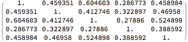
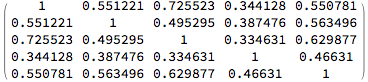
wincorr = Correlation[Transpose[%]];
wincorr // MatrixForm
{0.0117992, 0.0127976, 0.0155371, 0.011966, 0.00891589}
Standard VaR calculation
Having defined the volatility and the correlation matrix based on past year data, we can calculate the parametric VaR easily. Assuming the normal distribution for the stock returns and 1 day VaR horizon, this can be defined as follows:
Individual stock VaR
indVar=-Sqrt[2] [Pi] [Sigma] erfc^-1(2 [Alpha]) where [Pi] = value of the investment = £1 million, [Sigma] = stock return volatility and [Alpha]= confidence level
ndinv = Refine[InverseCDF[NormalDistribution[0, \[Sigma]], \[Alpha]],
  0 < \[Alpha] < 1]
-Sqrt[2] [Sigma] InverseErfc[2 [Alpha]]
With 99% confidence and each stock volatility calculated above
indvar = Table[
  10^6 ndinv /. {\[Alpha] -> 0.99, \[Sigma] -> volwin[[i]]}, {i, size}]
Total[%]
BarChart[indvar, ChartStyle -> "Rainbow",
 PlotLabel -> Style["Individual stock 1 day VaR", 16],
 ChartLegends -> stocks]
{27449.1, 29771.8, 36144.6, 27837.1, 20741.5}
141944.
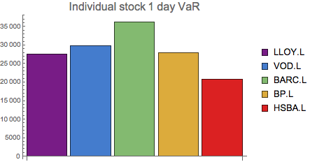
We can see the highest individual VaR for Barclays and the lowest for HSBC. This is consistent with the individual stock volatilities observed above.
Portfolio VaR
Formula-wise this is equivalent to: portVaR=Sqrt[indVar^T.[CapitalSigma].indVar]
baseportVaR = Sqrt[indvar.wincorr.indvar]
104226.
One can see that the portfolio VaR < [Sum] individual VaRs due to diversification effect. Portfolio features reduce the sum of individual VaR by almost £40,000.
The 1 day total portfolio VaR is £104k or 2.2% of the portfolio's value
Stressed VaR
VaR is a function driven primarily by volatility of return. In portfolio context there is another factor - correlations. When stressing VaR, one has to think about stress extension to both parameters.
Historical scenario of past crisis
This is the most frequently used method to handle stress testing. Having available data for the entire period makes this selection simple. Looking at the historical volatility graph, it is obvious that the volatility peaked in 2009 - 2010. We therefore select this period for our stress testing.
tswin = {{2009, 3, 1}, {2010, 3, 1}};
retwin = TimeSeriesWindow[dret, tswin];
volwin = Table[
  Mean[MovingMap[StandardDeviation, retwin[[i]], {60, "Day"}][[All,
    2]]], {i, size}]
Table[retwin[[i, All, 2]], {i, size}];
wincorr = Correlation[Transpose[%]];
wincorr // MatrixForm
{0.0412017, 0.013961, 0.0342192, 0.0138671, 0.0187612}
We can now see very different values for both - the volatilities and the correlation matrix. To compute the stressed VaR, all we need is just to replace the standard VaR set with the stress period data:
indSTvar =
 Table[10^6 ndinv /. {\[Alpha] -> 0.99, \[Sigma] -> volwin[[i]]}, {i,
   size}]
Total[%]
BarChart[indSTvar, ChartStyle -> "Rainbow",
 PlotLabel -> Style["Individual stock 1 day Stress VaR", 16],
 ChartLegends -> stocks]
{95849.5, 32478.1, 79605.9, 32259.8, 43645.}
283838.
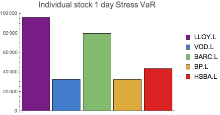
Consequently, the individual stocks stress VaR is very different from the standard VaR. For example, the Lloyds stressed VaR is almost 3 times higher than the standard VaR measure. Portfolio-level stressed VaR:
stressPortVaR = Sqrt[indSTvar.wincorr.indSTvar]
218471.
BarChart[{baseportVaR, stressPortVaR}, ChartStyle -> {Blue, Red},
 ChartLegends -> {"Std VaR", "Stress VaR"}]
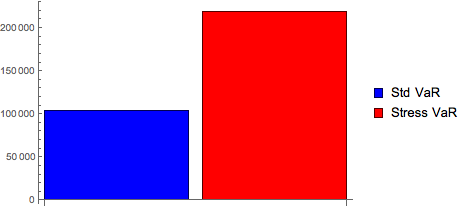
The portfolio 1 day stressed VaR has doubled under the stress scenario and represents £218k loss We can eventually choose any other period to see how the VaR behaves under different set of market parameters.
Inverse CDF method for stress scenarios - individual case
The calibration of historical volatility to the Johnson distribution enables us to explore alternative route for the stressed VaR generation. This can be described as Inverse CDF method.
If we assume that the return distribution is normal and the volatility of that return is calibrated to the Johnson unbounded distribution, we can obtain the stressed VaR metrics as a quantile of both distributions.
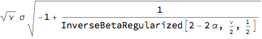
We are interested in the quantile value of the volatility to capture the stressed market sentiment. This can be easily achieved through the Inverse CDF function
invJD = Refine[
   InverseCDF[
    JohnsonDistribution [
     "SU", \[Gamma], \[Beta], \[Kappa], \[Nu]], \[Lambda]],
   0 < \[Lambda] < 1] // Simplify
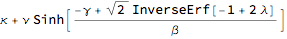
The VaR is then the composite value of the VaR formula and the quantiled volatility measure
stVaRNd = ndinv /. \[Sigma] -> invJD // Simplify
ndinv
The above formula is the parametric definition of the stressed VaR. The function operates on two quantile parameters: - VaR confidence level [Alpha] - Volatility 'stress' factor [Lambda]
The stressed VaR parametric model will behave as follows:
Plot3D[stVaRNd /. {\[Kappa] -> 0.006583, \[Nu] ->
    0.0002419, \[Gamma] -> -4.978, \[Beta] -> 1.07132}, {\[Alpha],
  0.5, 0.9}, {\[Lambda], 0.3, 0.75},
 ColorFunction -> "TemperatureMap", PlotLegends -> Automatic]
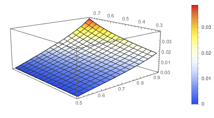
It is worth noting that the model is quite sensitive to the volatility stress factor [Lambda].
Probabilistic approach to stress VaR - portfolio context
Apart from stressing volatility parameter, we need to define the stressed correlation matrix. We propose simple multiplicative factor approach where the original matrix is multiplied by a positive number which increases the correlation coefficients in the matrix. This is consistent with market practice - in period of crisis there is a strong positive tendency for financial assets in the same class to move together. The function below does exactly this:
stressCM[cm_, f_] :=
 Table[If[cm[[i, j]] == 1, 1, Min[0.99, cm[[i, j]]*(1 + f)]], {i,
   size}, {j, size}]
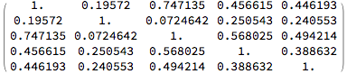
Applying 20% increase on the correlations of standard VaR produces the following CM:
stressCM[wincorr, 0.2] // MatrixForm
The matrix values are in line with the stressed matrix historical scenario of 2009-2010
To execute the computation we first generate the individual stressed VaR metrics using the Inverse CDF method:
indstressvar =
 Table[10^6 ndinv /. {\[Alpha] -> 0.99, \[Sigma] ->
     Mean[InverseCDF[edist[[i]], {0.5, 0.7, 0.9}]]}, {i, size}]
Total[%]
{86608., 37365.8, 82986.8, 41072.8, 41535.8}
289569.
And then obtain the portfolio VaR in the same way as in the standard case but with the stressed correlation matrix:
portstvar = Sqrt[indstressvar.stressCM[wincorr, 0.2].indstressvar]
232010.
The parametric stressed VaR number is similar to what we obtained when we applied the historical scenario method. This shows that the alternative probabilistic stressed VaR approach works well and can be easily applied in practical setting.
Extension of the stressed VaR concept
VaR with Student-T distribution
When we opt for the generalised Student-T distribution for stock returns, the standard VaR can be defined as:
StVaR = Refine[
   InverseCDF[StudentTDistribution[0, \[Sigma], \[Nu]], \[Alpha]],
   1/2 < \[Alpha] < 1] // Simplify
The extension to the stressed VaR is trivial:
StVaR /. \[Sigma] -> invJD

The formula is essentially the Student-T Stressed VaR expression
We need to calibrate the distribution to obtain the degrees of freedom value for each stock
edist2 = Table[
  EstimatedDistribution[dret[[i, All, 2]],
   StudentTDistribution[0, \[Sigma], \[Nu]]], {i, size}]
{StudentTDistribution[0, 0.0155062, 1.90416], StudentTDistribution[0, 0.0093817, 2.82662], StudentTDistribution[0, 0.0154996, 1.92631], StudentTDistribution[0, 0.00850414, 2.12496], StudentTDistribution[0, 0.00925811, 2.35383]}
stparam = List @@@ edist2
{{0, 0.0155062, 1.90416}, {0, 0.0093817, 2.82662}, {0, 0.0154996, 1.92631}, {0, 0.00850414, 2.12496}, {0, 0.00925811, 2.35383}}
The individual stocks VaR are then:
ststressind =
 Table[10^6 StVaR /. {\[Alpha] -> 0.99, \[Nu] ->
     stparam[[i, 3]], \[Sigma] ->
     Mean[InverseCDF[edist[[i]], {0.5, 0.7, 0.9}]]}, {i, size}]
Total[%]
{98371.2, 33623.8, 96266.1, 44665.5, 41708.4}
314635.
and the total portfolio VaR equals to:
Sqrt[ststressind.stressCM[wincorr, 0.2].ststressind]
253701.
The Student-T stressed VaR is higher than in the normal case which is in line with expectation, especially when the degree of freedom is < 4.
Conclusion
Parametric stressed VaR represents elegant and practical extension to the existing methods for stress testing. The main feature of this approach is ease of use and simplicity of application once the calibration dataset is available.
The parametric method can be applied to other probability distributions if one wants to test the parametric stressed VaR under different distributional assumptions. Student T approach is explicitly presented to demonstrate this case. Extension to other distributions is trivial since the stressed volatility with Inverse CDF can be easily applied in arbitrary setting.
 Attachments:


