Using a module is most often the hard way to solve a problem in Mathematica. Use functional composition. This kind of step-by step simulation is well represented as an "iterated function system". Nest and its relatives are powerful tools.
First, define the essential core of the random walk:
rwstep[x_] := x + RandomReal[{-1, 1}]
If a uniform distribution isn't desired, you can change this definition, of course. Test it:
In[2]:= NestList[rwstep, 0, 10]

Out[2]= {0, 0.401683, 1.20622, 0.250873, 1.19009, 2.16909, 2.02779, \
1.67653, 1.4804, 0.549813, 0.485389}
This works on scalers, but it's easy to make it work on multidimensional vectors:
SetAttributes[rwstep, Listable]
Test in 2D:
In[4]:= NestList[rwstep, {0, 0}, 10]

Out[4]= {{0, 0}, {-0.665343,
  0.145752}, {0.0847378, -0.468907}, {0.881671, -0.255809}, {1.23833, \
-0.367517}, {0.52246, 0.120586}, {0.152003, 0.621178}, {0.471109,
  1.31935}, {0.407214, 2.01076}, {0.785204, 2.99294}, {1.19189,
  3.26625}}
OK, I assume that your reference to "distance travelled in the xy plane" means that you want to terminate the random walk when it has traversed some particular Euclidean distance. That suggests Norm and NestWhileList are the appropriate tools:
rwd[d_] := NestWhileList[rwstep, {0, 0}, Norm[#] < d &]
Test it:
In[6]:= rwd[3]

Out[6]= {{0, 0}, {-0.338653, 0.701064}, {-0.884427,
  1.20091}, {-0.466393, 1.43251}, {-1.34926, 0.952485}, {-1.57566,
  1.02539}, {-0.623912, 0.559162}, {-0.603445,
  0.150985}, {-0.0936244, -0.436107}, {-0.721492, -1.41176}, \
{-1.19993, -2.24032}, {-0.423344, -2.61849}, {0.166061, -2.40501}, \
{-0.231736, -3.10079}}
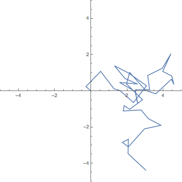
Now to make your plot:
ListPlot[rwd[5], {Joined -> True, PlotRange -> {{-5, 5}, {-5, 5}},
  AspectRatio -> 1}]

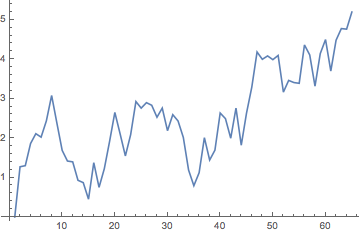
One nice thing about composing your problems as simple functions rather than writing complex modules is that you can easily take your functional factors and reuse them. For example, it's easy here to plot distance from origin versus time:
ListPlot[Map[Norm, rwd[5]], Joined -> True]

Note that this is a different simulation from the previous. If you want to extract multiple results from a single simulation, you'll want to save the list of points as the value of a symbol.