
Yesterday on March 25 2015 a Germanwings commercial passenger plane crashed in the French Alps tragically killing all 150 people onboard. While the exact circumstances of the crash are still unclear at the time of my writing this article, all of us who routinely fly inevitably ask how such a thing can happen. We start asking questions about air-traffic safety. In this post I will use Mathematica and an online data basis to look into the frequency of flight incidents. This website contains basically all the data that is required for this post. On the website there is a Java interface that allows us to search for certain types of incidents, which then are listed at the bottom of the page. Each event has its own url which is always of the form:
http://aviation.globalincidentmap.com/eventdetail.php?ID=XXXX
where the XXXX has to be replaced by a unique identifier. David Gathercole, a student of mine, who is also member of this community, has programmed a little webscaper to download incidents from the database:
scrapeSequence[from_, to_] :=
 scrapeSequence[to, from] = Prepend[ParallelTable[
    Flatten[string = ToString[i]; While[StringLength[string] < 5, string = "0" <> string];
     Quiet[{Take[#, 2 ;; -1 ;; 2] & /@ (Drop[#, 1] & /@ #)[[1, 1]], (Drop[#, 1] & /@ #)[[2, 1]]}] & /@ {Import[
         "http://aviation.globalincidentmap.com/eventdetail.php?ID=" <>string, "Data"][[3]]}], {i, Max[1, from], to},
    Method -> "CoarsestGrained"],{"Event Type", "Date Time", "Country", "City", "Latitude", "Longitude", "URL", "description"}]
Running this will take some time (~hours):
Quiet[data = scrapeSequence[1, 15185];]
Be careful with this command, because it will initiate many requests to the same server. If too many people run it, this could cause problems to the server, which needs to be avoided at all cost. Also, the data can only be used for research and teaching. I use the data for research and teaching and show here only some educational content. If you use this command you might breach their fair usage policy. The cases in the data base span the time period from 2009 to today. The following command extracts all geo positions of all incidents:
geopos = ToExpression@(Select[data, Length[#] == 8 &][[2 ;;, {5, 6}]]);
which we can plot with GeoRegionValuePlot:
GeoRegionValuePlot[GeoPosition[#] -> 1 & /@ geopos, ColorFunction -> "Rainbow" , GeoBackground -> "ReliefMap", ImageSize -> Full, PlotLegends -> None, GeoRange -> "World"]
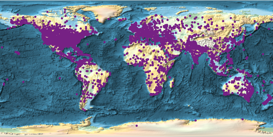
The image shows 15146 incidences. This generates a list of all of them in several categories:
(data[[2 ;;, 1]] // Tally) // TableForm
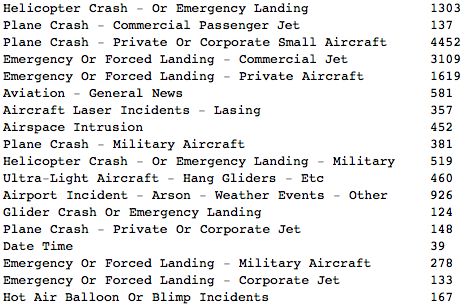
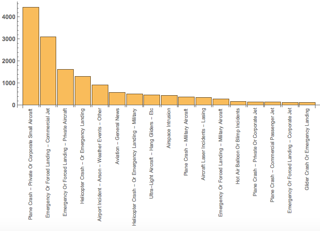
It becomes probably clearer in a BarChart:
BarChart[Reverse[SortBy[data[[2 ;;, 1]] // Tally, Last]][[1 ;; -2, 2]], ChartLabels ->
  Placed[Rotate[#, Pi/2 // N] & /@ (Reverse[SortBy[data[[2 ;;, 1]] // Tally, Last]][[1 ;; -2, 1]]), Axis],
 LabelStyle -> Directive[Bold, Medium], AspectRatio -> 1/3, ImageSize -> Large]
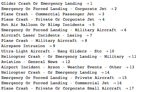
To get a more differentiated representation we will mark different events with different colours:
rules = #[[1]] -> #[[2]] & /@ Transpose[{SortBy[Tally[data[[2 ;;, 1]]], Last][[2 ;;, 1]], Range[17]}]
Now we can clean up the data and plot this like so:
incidents = Replace[Select[data, Length[#] == 8 &][[2 ;;, {1, 5, 6}]], rules, {2}];
GeoRegionValuePlot[GeoPosition[#[[{2, 3}]]] -> #[[1]] & /@ ToExpression[incidents],
 ColorFunction -> "Rainbow" , GeoBackground -> "ReliefMap", ImageSize -> Full, PlotLegends -> None, GeoRange -> "World"]
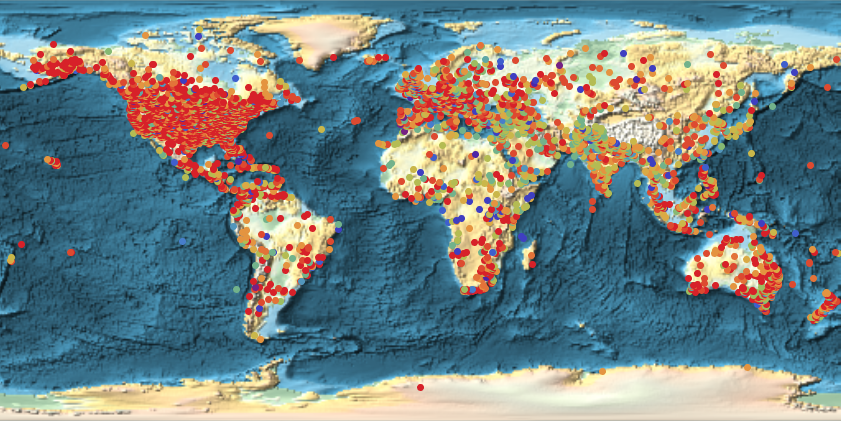
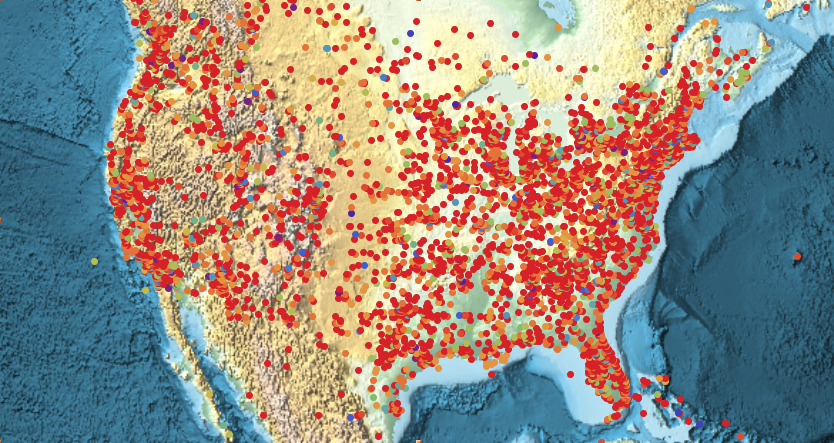
We see that there are many more cases in the US and Europe. This might be because of a higher level of reporting on these incidents. The same plot for the US shows some interesting features:
GeoRegionValuePlot[GeoPosition[#[[{2, 3}]]] -> #[[1]] & /@ ToExpression[incidents],
 ColorFunction -> "Rainbow" , GeoBackground -> "ReliefMap", ImageSize -> Full, PlotLegends -> None, GeoRange -> Entity["Country","UnitedStates"]]
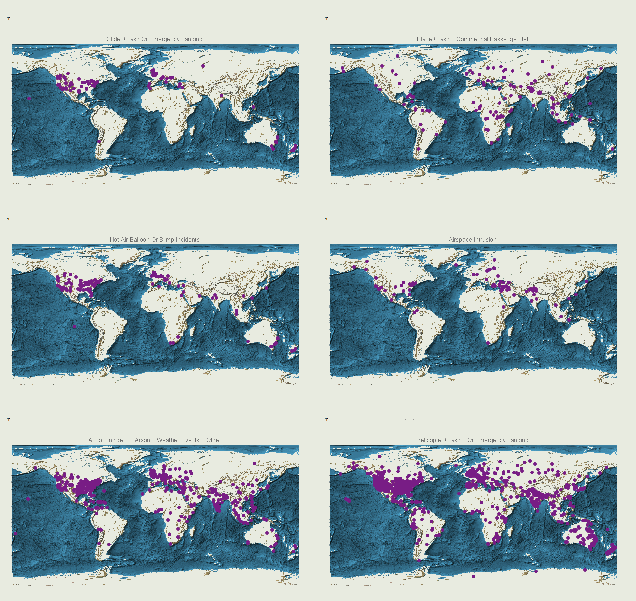
We can also look at the global cases by type:
Manipulate[GeoRegionValuePlot[#[[2]] & /@ (Select[timedata, #[[2, 2]] == m &]),
  ColorFunction -> "Rainbow" , GeoBackground -> "ReliefMap", ImageSize -> Large, PlotLegends -> None, GeoRange -> "World", PlotLabel -> rules[[m, 1]]], {m, 1, 17, 1}]
We can now also look at the temporal distribution of the incidents. We could use a function like this one:
Interpreter["DateTime"][#] & /@ data[[2 ;; 100, 2]]
to extract the time, but this one is much (!!!) faster:
dates = SemanticImport[Export["~/Desktop/dates.csv", Select[data, Length[#] == 8 &][[2 ;;, 2]]]];
We can put the information we need into one variable:
timeincidents = Transpose[{dates[[All, 1]] // Normal, GeoPosition[#[[{2, 3}]]] -> #[[1]] & /@ ToExpression[incidents]}];
timedata = SortBy[timeincidents, 1];
The first couple of entries look like this:

They tell me the date/time, the GeoPosition and the type of incident. The following command generates the frames for an animation:
Monitor[For[k = 1, k <= 57, k++,
  Export["~/Desktop/AirTrafficInc/frame" <> ToString[1000 + k] <> ".gif", GeoRegionValuePlot[#[[2]] & /@
     timedata[[-1200 + 20 k ;; -1180 + 20 (1 + k)]], ColorFunction -> "Rainbow" , GeoBackground -> "ReliefMap",
    ImageSize -> Large, PlotLegends -> None, GeoRange -> "World"]]],k]
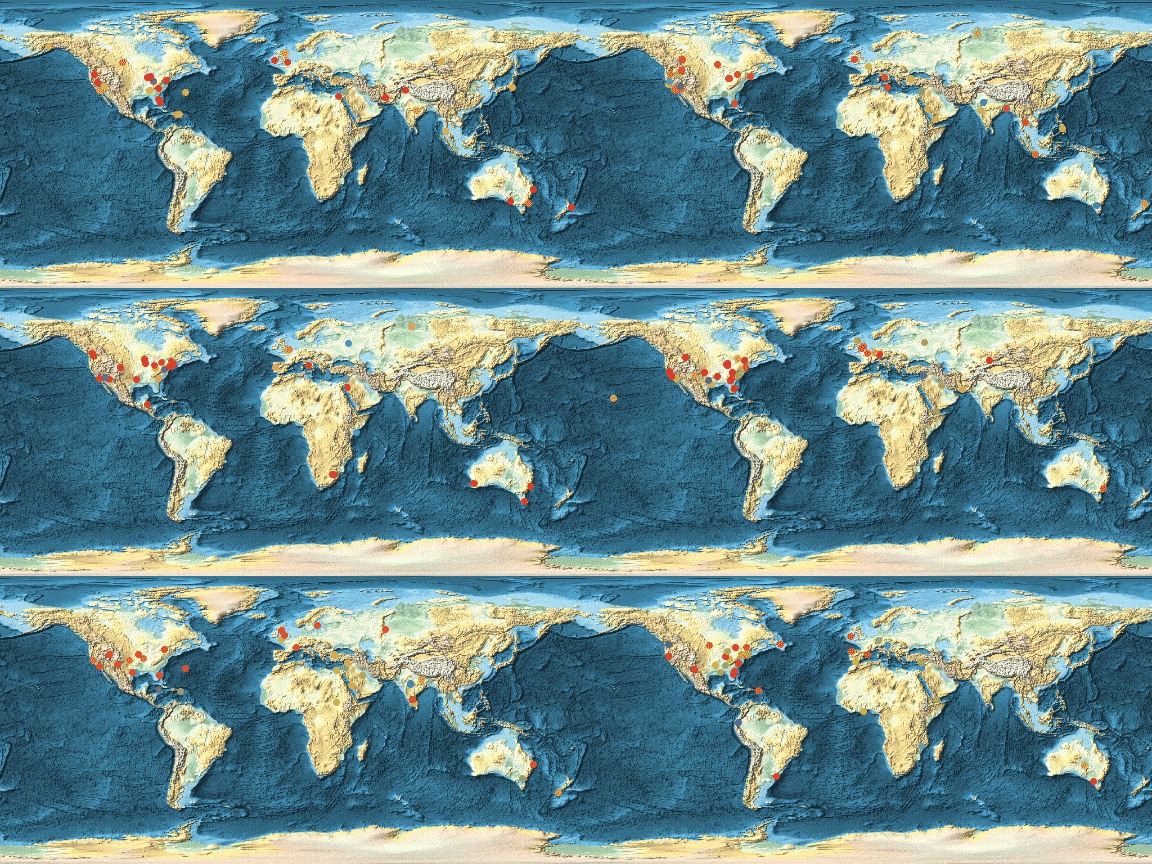
I use a terminal command to generate the animation but you can also directly export the frames as a gif. This is the result:
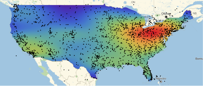
Borrowing some really great ideas from Michael Trott's blog post on beer we can also calculate heat maps for the distribution of say crashes. Here I demonstrate that for the US only.
projection = {"LambertAzimuthal", "Centering" -> GeoPosition[{37.1558, -95.883}]};
datacoords = GeoGridPosition[#, projection][[1]] & /@
   Flatten[List @@@ Select[timedata, (#[[2, 2]] == 17 || #[[2, 2]] == 14 || #[[2, 2]] == 11 || #[[2, 2]] == 8 || #[[2, 2]] == 4 || #[[2, 2]] == 3 || #[[2, 2]] == 1) &][[All, 2, 1]], 1];
We now restrict to cases in the US (GeoWithinQ is too slow for this):
datacoordsusa = Select[datacoords, (24.9382 < #[[1]] && #[[1]] < 49.37 && -67 > #[[2]] && #[[2]] > -124) &];
where you can get the coordinates intervals from:
GeoBoundingBox[Entity["Country", "UnitedStates"]]
Ok. Next we calculate the distribution:
crashDensityDistribution = SmoothKernelDistribution[RandomChoice[datacoordsusa, 1000], "Oversmooth"]
Next then we plot that:
cplot = ContourPlot[PDF[crashDensityDistribution, {y, x}],
  Evaluate@Flatten[{x, {#[[1, 1, 2]], #[[2, 1, 2]]} &@
      GeoBoundingBox[Entity["Country", "UnitedStates"]]}],
  Evaluate@Flatten[{y, {#[[1, 1, 1]], #[[2, 1, 1]]} &@
      GeoBoundingBox[Entity["Country", "UnitedStates"]]}],
  ColorFunction -> "Rainbow", Frame -> False, PlotRange -> All,
  Contours -> 205, MaxRecursion -> 2,
  ColorFunction -> ColorData["TemperatureMap"],
  PlotRangePadding -> 0, ContourStyle -> None]
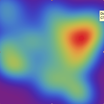
Overlaying that to the map of the US gives:
GeoGraphics[{GeoStyling[{"GeoImage", cplot}],
  Polygon[Entity["Country", "UnitedStates"]], Black, Opacity[1], PointSize[0.001],
  Point[Reverse /@ RandomChoice[datacoordsusa, 3500]]}, GeoRange -> Entity["Country", "UnitedStates"]]
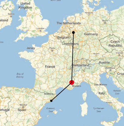
On the incidents website you also find all the data for the Germanwings plane:
germanwings = Import["http://aviation.globalincidentmap.com/eventdetail.php?ID=15185", "Data"]

The following map lists the waypoints. The flight was from Barcelona and scheduled to land in Duesseldorf (both marked in black). The crash site is marked in red.
GeoGraphics[{GeoStyling[Opacity[1]], Red, Opacity[1],
  GeoDisk[geopos[[-1]], Quantity[40, "Kilometers"]], Black,
  GeoDisk[Entity[
    "City", {"Dusseldorf", "NorthRhineWestphalia", "Germany"}],
   Quantity[20, "Kilometers"]],
  GeoDisk[Entity["City", {"Barcelona", "Barcelona", "Spain"}],
   Quantity[20, "Kilometers"]], Thickness[0.005],
  GeoPath[{EntityValue[
     Entity["City", {"Barcelona", "Barcelona", "Spain"}],
     "Coordinates"], geopos[[-1]],
    EntityValue[
     Entity["City", {"Dusseldorf", "NorthRhineWestphalia",
       "Germany"}], "Coordinates"]}, "Rhumb"]},
 GeoRange -> Quantity[1000, "Kilometers"],
 GeoProjection -> "Mercator"]
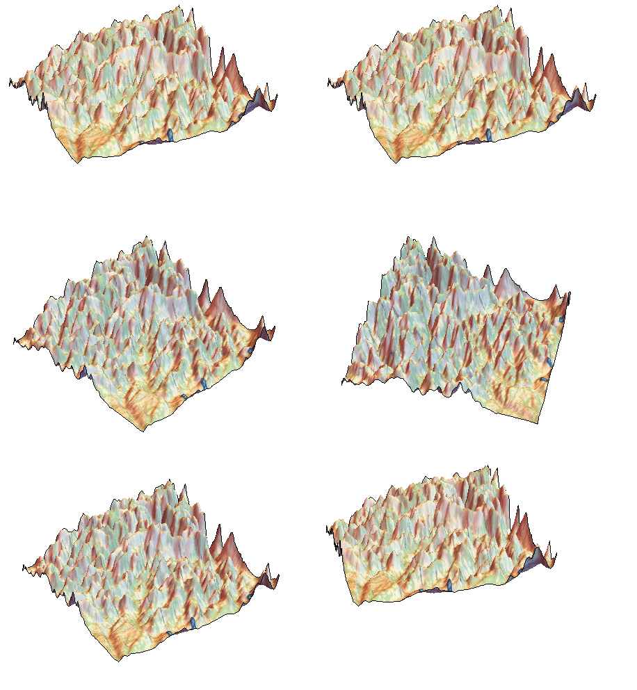
The region where the plane crashed is very mountainous:
dataelevation = GeoElevationData[GeoBoundingBox[GeoDisk[geopos[[-1]], Quantity[40, "Kilometers"]]]];
ListPlot3D[dataelevation, Mesh -> None, PlotStyle -> Texture[Image[GeoGraphics[GeoBoundingBox[GeoDisk[geopos[[-1]], Quantity[40, "Kilometers"]]],GeoBackground -> "StreetMap"]]], Boxed -> False, Axes -> False]
I hope that the cause of the crash will be determine swiftly and that similar disasters can be avoided in the future.
The following function:
Select[timedata, (#[[2, 2]] == 17 || #[[2, 2]] == 14 || #[[2, 2]] == 11 || #[[2, 2]] == 8 || #[[2, 2]] == 4 || #[[2, 2]] == 3 || #[[2, 2]] == 1) &] // Length
shows that there are 7064 cases in the database since 2009.
Select[timedata, (#[[2, 2]] == 3) &] // Length
counts the crashes of commercial passenger planes; in the data base there are 137 in 6 years or so - that would be about 22.8 per year, which is more than I would have expected. The number of course does not tell us the number of fatalities. Three million people fly every day on commercial aircraft alone. Google states:
Commercial jet aviation is an exceptionally safe way to get from here to there. More than three million people around the world fly safely on commercial aircraft every day. In 1998, the world's commercial jet airlines carried approximately 1.3 billion people on 18 million flights while suffering 10 fatal accidents.
I hope that this post helps to show how Mathematica might help to make up your mind about whether to fly or not.
Best wishes,
Marco