We extend the discussion on machine learning one step further and focus on predictive analysis offered in the ML domain. Prediction builds on classification and clustering techniques discussed previously and uses pattern detection and similarity features in data to estimate the future outcome. This is particularly relevant to finance where the ability of data groups to predict the values of less-liquid instruments is of high interest. We demonstrate the prediction using CDS data and show the application of non-regression models as superior methods for predictive analysis.

Introduction

Classification and clustering which we discussed in previous installments naturally extends into another field of data mining - prediction. It is well-known that there will be limited benefit of massive amount of data collection if the data cannot be analysed, decomposed into signals and used to predict future behaviour. Therefore, data analysis in statistics and econometrics can be broken down into four major categories: (i) prediction, (ii) summarisation, (iii) estimation, and (iv) hypothesis testing. Machine learning , as we have stated previously, focuses primarily at data organisation and prediction. However, closely related field is also data summarisation where pattern finding in the data - covered by the classification - is of primary interest. Machine learning is therefore about developing high-performance computer systems that can provide useful predictions in the presence of challenging computational constraints. This whole area of data processing is today routinely described as data science, which is primarily looks at both prediction and summarisation, but also extends into data manipulation, visualization, and other similar tasks.

In pure statistical terms, the prediction problem reduces to finding conditional distribution of some variable y given some other variables $x= (x_ 1,x_ 2,...x_n)$. In data science methodology, variables x are called 'predictors' or 'features'. The prediction point y is generally the highest value (mean) of the calibrated conditional distribution.

Prediction basics

Much of applied econometrics, economics and finance is concerned with detecting and summarising relationships in the data. The most common tool is (linear) regression analysis. Machine learning offers richer set of tools that can usefully summarise various sorts of nonlinear relationships in the data. We will focus on these regression-like tools because they are the most natural for economic and financial applications.

The objective of prediction is to find some function that gives a good estimate of y as function of x. In machine learning context the data we work with are generally considered independent and identically distributed. They may be 'fat' which implies more predictors relative to observations or 'tall' which indicated many observations relative to predictors.

When we build prediction routines, we start with some observation of y and x and then want to obtain the predicted point for the new value x .'Good' prediction involves finding a function that minimises some error estimation. Sum of squared residuals, mean residual value are generally the most frequently used tools in this context. Tradition all method to solve this problem is regression - typically linear or logistic However, machine learning offers better options especially when there is a lot of data available. These include trees, nearest neighbors, random forests or neural networks.

Working with predictions

Objective of prediction routines is to find good out-of-sample estimation to the data. This task is not always trivial and regressions are generally known to be 'weak' around out-of-sample predictions. This is generally known as 'overfitting' problem. Machine learning addresses this problem through:

• Regularisation - preference is given to simpler models
• Dataset division into (i) training and (ii) testing sets
• Cross-validation of the dataset and the model

Prediction relation to other data mining techniques

Irrespective of the method structure, there is a common confusion between explanatory and predictive models. In a predictive model only the model's accuracy is important and the structure of the model is relatively unimportant, as long as it is robust. In general, models become more robust as the number of predictors declines, and hence there is a greater tendency towards parsimony in predictive models, often using variable selection algorithms.

However, if a model is developed for explanatory purposes, the identity and weights of the predictors is the most important part of the model because these are used to infer the nature of the relationship between the class and the values of the predictor variables.

The contribution made by the predictors is obviously most important in an explanatory, rather than a predictive, model. In predictive models the role of predictors is less important than the accuracy of the prediction. Consequently, the use of variable selection routines that produce a more parsimonious model are generally more acceptable in predictive models.

Prediction in Finance

The advantages offered by machine learning are well suited for the data analysis in finance, particularly when the larger datasets are available. For years, the regression technique was dominant in economics and finance on the premise of limited amount of data. However,nowadays, in data-rich era, there is no reason not to start applying machine learning methods more frequently in economic and financial industries with data separation or the use of validation sets.

Problem definition

Let's define the following problem: we have available set of actively traded and liquid CDS rates ( 5 years of daily rates) that we would like to use for prediction of lesser liquid CDS. These types of problem frequently occur in the credit or equity markets where liquidity factor drives certain instruments into specific categories.

• 3 CDS will serve as features
• We split the data into three sets: (i) training, (ii) testing and (iii) validation
• We apply several predictive routines to obtain the future value in the out-of-sample domain

Data generation

vols = {0.01, 0.008, 0.011, 0.008};
crl = ({
    {1, 0.35, 0.45, 0.36},
    {0.35, 1, 0.43, 0.32},
    {0.45, 0.43, 1, 0.46},
    {0.36, 0.32, 0.46, 1}
   });
cm = Table[vols[[i]]*vols[[j]]*crl[[i, j]], {i, 1, Length[vols]}, {j, 1, Length[vols]}]

{{0.0001, 0.000028, 0.0000495, 0.0000288}, {0.000028, 0.000064, 0.00003784, 0.00002048}, {0.0000495, 0.00003784, 0.000121, 0.00004048}, {0.0000288, 0.00002048, 0.00004048, 0.000064}}

init = {0.55, 0.72, 1.25, 1};
mn = MultinormalDistribution[{0, 0, 0, 0}, cm];
data = Accumulate[Prepend[RandomVariate[mn, 1500], init]];
ListLinePlot[Transpose[data], 
 PlotLegends -> {"cds 1", "cds 2", "cds 3", "cds 4"}, 
 PlotLabel -> Style["CDS of observed series", 15]]

traindata = data[[;; 600]];
validata = data[[601 ;; 900]];
testdata = data[[901 ;;]];

trainset = 
  Table[Drop[traindata, None, -1][[i]] -> 
    Flatten[Take[traindata, All, -1]][[i]], {i, 1, Length[traindata]}];
testset = 
  Table[Drop[testdata, None, -1][[i]] -> 
    Flatten[Take[testdata, All, -1]][[i]], {i, 1, Length[testdata]}];
validset = 
  Table[Drop[validata, None, -1][[i]] -> 
    Flatten[Take[validata, All, -1]][[i]], {i, 1, Length[validata]}];

{ListLinePlot[Transpose[traindata], 
  PlotLegends -> {"cds 1", "cds 2", "cds 3", "cds 4"}, 
  PlotLabel -> Style["Training data", 15]], 
 ListLinePlot[Transpose[testdata], 
  PlotLegends -> {"cds 1", "cds 2", "cds 3", "cds 4"}, 
  PlotLabel -> Style["Testing data", 15]], 
 ListLinePlot[Transpose[validata], 
  PlotLegends -> {"cds 1", "cds 2", "cds 3", "cds 4"}, 
  PlotLabel -> Style["Validation data", 15]]}

We can investigate the predictors separately by looking at histogram of the training data:

edata = Transpose[Drop[traindata, None, -1]];
{Histogram[edata[[1]], 20, ChartStyle -> "Pastel", 
  PlotLabel -> "Feature 1"], 
 Histogram[edata[[2]], 20, ChartStyle -> "Rainbow", 
  PlotLabel -> "Feature 2"], 
 Histogram[edata[[3]], 20, ChartStyle -> "NeonColors", 
  PlotLabel -> "Feature 3"]}

Setting the predictors

Having defined the training, testing and validation sets, we can now set up the prediction model:

Take[trainset, 10]

{{0.55, 0.72, 1.25} -> 1, {0.571876, 0.719578, 1.24021} -> 0.997824, {0.577651, 0.719425, 1.23595} -> 1.00456, {0.573492, 0.706407, 1.23029} -> 1.00455, {0.564589, 0.721109, 1.2309} -> 0.999223, {0.582398, 0.73248, 1.2497} -> 1.00538, {0.583999, 0.727467, 1.25179} -> 0.999114, {0.592003, 0.721993, 1.24155} -> 0.990911, {0.592474, 0.718474, 1.23417} -> 0.985031, {0.603327, 0.710775, 1.22836} -> 0.98689}

Given the size of the training set we select Random Forest algorithm for prediction routine

pred = Predict[trainset, ValidationSet -> validset, Method -> "RandomForest", PerformanceGoal -> "Quality"]

and obtain the information on the model

PredictorInformation[pred]

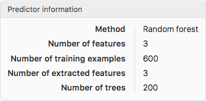
The automatic routine selects the Random Forest as the most optimal algorithm for this task

Conditional distribution

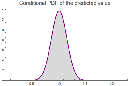
We can obtain the information about the distribution of the predicted value:

dist = pred[Drop[init, -1], "Distribution"]

NormalDistribution[1.00262, 0.0288765]

It is confirmed that the predicted value is normally distributed with mean close to the and low volatility.

PDF[dist, x]
Plot[PDF[dist, x], {x, 0.8, 1.25}, PlotStyle -> {Thick, Purple}, 
 FillingStyle -> LightGray, Filling -> Axis, 
 PlotLabel -> Style["Conditional PDF of the predicted value", 15]]

13.8155 E^(-599.627 (-1.00262 + x)^2)

Testing predictor accuracy

We may be interested to check how accurate the predictor works relative to the original data.

plotdata = Drop[traindata, None, -1];
adata = Transpose[Take[traindata, All, -1]] // Flatten;
pdata = Table[pred[plotdata[[i]]], {i, 1, Length[traindata]}];
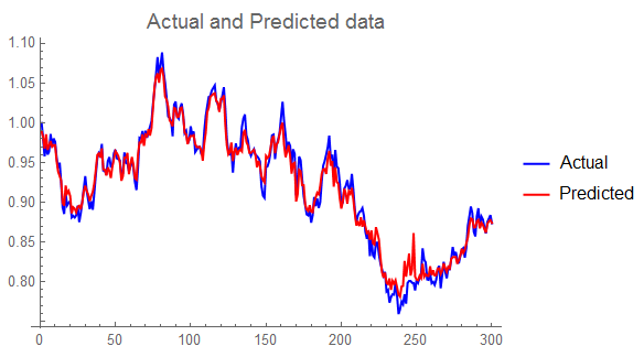
ListLinePlot[{adata, pdata}, 
 PlotLabel -> Style["Actual and Predicted data", 15], 
 PlotLegends -> {"Actual", "Predicted"}, PlotStyle -> {Blue, Red}]

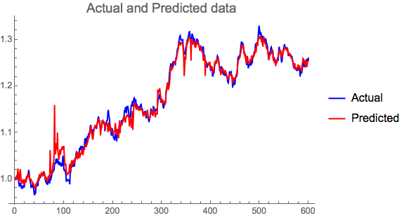
We can see that the predictor replicates the original data quite well.

Verification with Testing data set

We can test and validate the classifier with the <ClassifierMeasurements> command. For example, we can used the testing set defined above and look at its subset:

Take[testset, 10]

{{0.485579, 0.621485, 1.15959} -> 1.0466, {0.485904, 0.630628, 1.15086} -> 1.04336, {0.477018, 0.618847, 1.14833} -> 1.04416, {0.492894, 0.627871, 1.15071} -> 1.04294, {0.496431, 0.626622, 1.15025} -> 1.04363, {0.501258, 0.629071, 1.14728} -> 1.04505, {0.506147, 0.630316, 1.15071} -> 1.05803, {0.492122, 0.627663, 1.15387} -> 1.05949, {0.485113, 0.626491, 1.16395} -> 1.0621, {0.476587, 0.632491, 1.16424} -> 1.05147}

pm = PredictorMeasurements[pred, testset]

The classifier returns the correct class group ping for all categories with high precision.

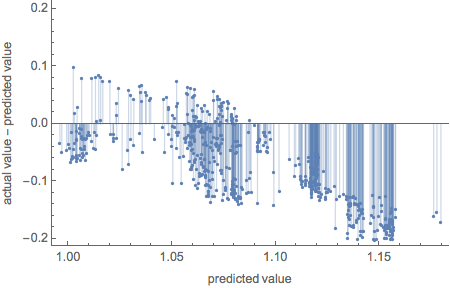
• Resting of residuals

  pm["ResidualPlot"]
  

• Testing of comparison

  pm["ComparisonPlot"]
  

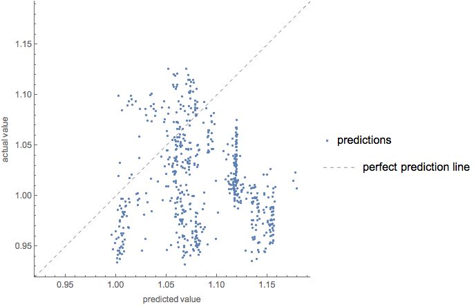
Predictor sensitivity to the features variability

We look how the predictor reacts to the features input w.r.t. calibrated conditional distribution

{Plot[pred[{x, 0.7, 1.25}], {x, 0.4, 0.7}, PlotStyle -> Blue, 
  Filling -> Axis, FillingStyle -> LightYellow, 
  PlotLabel -> Style["1st CDS sensiitivtiy", 13]], 
 Plot[pred[{0.6, x, 1.25}], {x, 0.6, 0.8}, PlotStyle -> Magenta, 
  Filling -> Axis, FillingStyle -> LightGray, 
  PlotLabel -> Style["2nd CDS sensiitivtiy", 13]], 
 Plot[pred[{0.6, 0.7, x}], {x, 1.1, 1.3}, PlotStyle -> Green, 
  Filling -> Axis, FillingStyle -> LightBrown, 
  PlotLabel -> Style["3rd CDS sensiitivtiy", 13]]}

As charts above suggest, each feature affects the predictor differently:

• 1st CDS both decreases and increases the predicted value as the CDS move upwards
• 2nd CDS increased the predicted value on the entire range, however the degree of impact varies
• 3rd CDS is impact less on the lower side of the range and then increases the predicted CDS rate

Predicting outcomes with new data

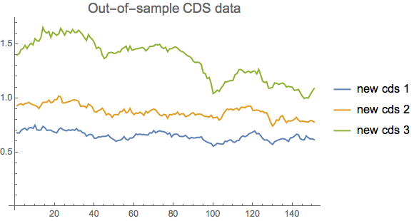
We now apply the predictor to the out-of-sample data based on the specification above:

• Define new covariance matrix

  tvols = {0.015, 0.02, 0.03};
  tcorr = ({
      {1, 0.4, 0.5},
      {0.4, 1, 0.45},
      {0.5, 0.45, 1}
     });
  tcm = Table[ tvols[[i]]*tvols[[j]]*tcorr[[i, j]], {i, 1, Length[tvols]}, {j, 1,  Length[tvols]}]
  

{{0.000225, 0.00012, 0.000225}, {0.00012, 0.0004, 0.00027}, {0.000225, 0.00027, 0.0009}}

• Generate the new CDS data for each feature

  newinit = {0.68, 0.93, 1.4};
  mn = MultinormalDistribution[{0, 0, 0}, tcm];
  tdata = Accumulate[Prepend[RandomVariate[mn, 150], newinit]];
  ListLinePlot[Transpose[tdata], 
   PlotLegends -> {"new cds 1", "new cds 2", "new cds 3"}, 
   PlotLabel -> Style["Out-of-sample CDS data", 15]]
  

newdata = Table[predauto[tdata[[i]]], {i, 1, Length[tdata]}];
ListLinePlot[newdata, PlotTheme -> "Web", 
 PlotLabel -> 
  Style["Predicted value of CDS for put-of-sample input", 15]]
![enter image description here][14]

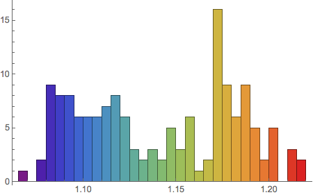
We have obtained the new predicted data which we can investigate further:

• Data distribution

  edist = SmoothKernelDistribution[newdata]
  

    Plot[PDF[edist, x], {x, 1, 1.3}, 
     PlotLabel -> "Probability density of the predicted value", 
     Filling -> Axis, PlotRange -> All]

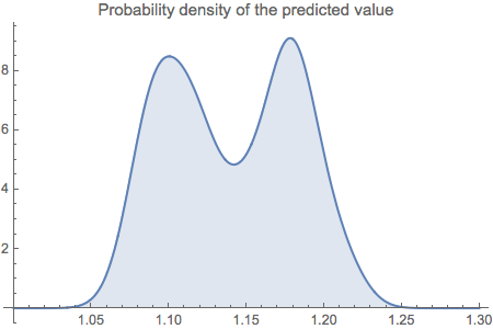
This is the estimated probability density from the predicted data.

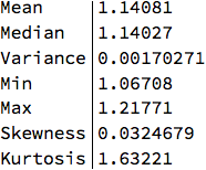
• Descriptive statistics

  stats = {Mean, Median, Variance, Min, Max, Skewness, Kurtosis};
  TableForm[Through[stats[newdata]], TableHeadings -> {stats, None}]
  

• Histogram

  Histogram[newdata, 25, ChartStyle -> "Rainbow"]
  

Alternative prediction methods

We can test other prediction methods available in Predict command:

• Linear regression

  plinreg = 
   Predict[trainset, ValidationSet -> validset, 
    Method -> "LinearRegression", PerformanceGoal -> "Quality"]
  

    pmlin = PredictorMeasurements[plinreg, testset];
    pmlin["ResidualPlot"]

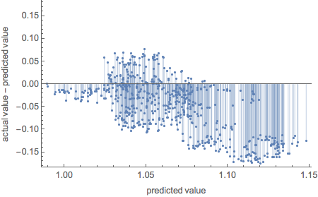
    plinreg[Drop[init, -1], "Distribution"]

NormalDistribution[1.09925, 0.0769071]

We observe higher predicted value and higher volatility relative to Random Forest

• NearestNeighbors

  pnn = Predict[trainset, ValidationSet -> validset, 
    Method -> "NearestNeighbors", PerformanceGoal -> "Quality"]
  

    pnntest = PredictorMeasurements[pnn, testset];
    pnntest["ResidualPlot"]

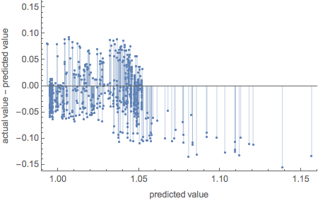
pnn[Drop[init, -1], "Distribution"]

NormalDistribution[0.982606, 0.0304784]

NearestNeighbors produces excellent fit to the data, but significantly higher volatility

• Neural network

  pneural = 
   Predict[trainset, ValidationSet -> validset, 
    Method -> "NeuralNetwork", PerformanceGoal -> "Quality"]
  

    pneuraltest = PredictorMeasurements[pneural, testset];
    pneuraltest["ResidualPlot"]

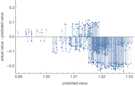
pneural[Drop[init, -1], "Distribution"]

NormalDistribution[0.974001, 0.0461196]

Reasonable fit to the data but with higher volatility than Random Forest.

Conclusion

Prediction is useful technique for finding relationship in data, especially if we have at our disposal larger set of data. Machine learning comes particularly handy in detecting patterns better than traditional linear model. The tools and methods such as decision trees, neutral networks or nearest neighborhood offer more flexibility to find complex relationship

Prediction as a method to estimate outcome from supporting features naturally offers practical solutions to finance and economics where the estimation can be quite valuable. Market data generation, growth rates forecast, marketing campaign model testing or inflation prediction are just few examples where machine learning with prediction focus becomes essential tool for decision making.Richer contents and better prediction ability makes machine learning more powerful than traditional regression techniques.