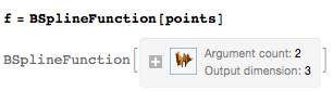
You can use the BSplineFunction to generate the interpolation function of the B-spline surface and project it onto either x-z plane or y-z plane. I use the same control points in your original input:

You can plot the surface with the ParametricPlot3D function. The result should be similar to yours. If you wrap the plot function with Manipulate, you can see the partial plot:

Manipulate[
 ParametricPlot3D[f[u, v], {u, 0, k}, {v, 0, 1}, Mesh -> None, 
  PlotRange -> {{1, 10}, {0, 20}, {-0.5, 0.5}}, 
  BoxRatios -> {1, 2, 0.4}, PlotPoints -> 20],
 {k, 0.005, 1}]

Use the Table function to generate a list of points on the surface and we can find the projection by the following code:

ls = Table[f[k, v], {k, 0, 1, 0.01}, {v, 0, 1, 0.01}];
yzplan = Transpose@Map[{#[[1]], #[[3]]} &, ls, {2}];
xzplan = Map[{#[[2]], #[[3]]} &, ls, {2}]; (* the length is 101*)

Use the Manipulate to show the shadow and its original curve on the B-spline surface:

Manipulate[
 Show[plt1, ListPlot[xzplan[[k]], PlotStyle -> Black]],
 {k, 1, 101, 1}, 
 Initialization :> (plt1 = 
    ListLinePlot[xzplan, PlotRange -> All, 
     PlotStyle -> Directive[Thin, Opacity[0.3]], Filling -> Axis, 
     FillingStyle -> Opacity[0.2]]) ]

Similarly, on the x-z plane we have

Manipulate[
 Show[plt2, ListPlot[yzplan[[k]], PlotStyle -> Black]],
 {k, 1, 101, 1}, 
 Initialization :> (plt2 = 
    ListLinePlot[yzplan, PlotRange -> All, 
     PlotStyle -> Directive[Thin, Opacity[0.3]], Filling -> Axis, 
     FillingStyle -> Opacity[0.2]]) ]

Please find the attached notebook for codes.

Attachments: