The following is a modelling project produced by Hannah Higgins, Mark McDowell and James Milne as part of the final year of our honours degree in mathematics. We'd like to take the opportunity to share our work, which was carried out using Mathematica...
The idea of predicting football results is a fascinating one, and at the same time seems implausible. After all football is supposedly unpredictable - scores can vary greatly game by game and the team perceived to be stronger does not always emerge victorious. Inspired by the book How to Take a Penalty: The hidden mathematics of sport by Rob Eastaway and John Haigh, we aimed to use probabilities to produce a mathematical model using Mathematica which was capable of giving predictions for games in the 2013/14 Premier League season with some level of accuracy.
To forecast future results we needed to interpret past results. Note that, unlike in international football, fortunes in club football can fluctuate massively over short periods of time. For example, Manchester City were a mid-table team in the mid 2000s, yet following a takeover of the club in 2008, hundreds of millions of pounds has been invested, thus propelling Manchester City up to the top end of the Premier League in recent seasons. Therefore it would be ill-advised to take into account too many seasons when choosing past results to interpret. We chose to use only the season prior to the one being forecast, namely the 2012/13 season.
Data on past results can easily be found online.
data1213=Import["http://www.soccerstats.com/results.asp?league=england_2013","Data"];
Data cleaning was performed to remove irrelevant information, leaving only details of the teams and their respective scores for each of the 380 games of the season. This data was then exported as an XML file which can be accessed without an internet connection (see attached file).
Drop[Drop[Cases[data1314,{_,_,_,_,_},Infinity],None,{1,2}],None,{3}];
  Drop[%,{1}];
  Table[StringSplit[%[[i]],"-"],{i,1,380}];
  resultsdata1213=Transpose[{StringTrim[%[[All,1,1]]],ToExpression[StringTrim[%[[All,2,1]]]],StringTrim[%[[All,1,2]]],ToExpression[StringTrim[%[[All,2,2]]]]}];
  Export["result201213.xml",resultsdata1213]];
This webpage is no longer accessible so this code actually fails. However we can import the XML file which was created prior to the loss of the webpage, and check the scores are defined as integers, before extracting the home and away goals data as well as removing whitespace from the team entries.
resultsdata=Import["results201213.xml"];
Head[resultsdata[[1,2]]]
Head[resultsdata[[1,4]]]
hgoals=resultsdata[[All,2]];
agoals=resultsdata[[All,4]];
resultsdata[[All,1]]=StringTrim[resultsdata[[All,1]]];
resultsdata[[All,3]]=StringTrim[resultsdata[[All,3]]];

Making predictions involved the analysis of probabilities of certain scores based on the results from the 2012/13 season. Therefore, it was necessary to choose a probability distribution that fitted the process of goals being scored. Considering this over a 90 minute game we observed that this is a stochastic process. By counting the number of goals over this time period the Poisson distribution should be possible to implement with expectation given by the mean number of goals per game. However, to verify this claim some checks needed to be performed. Firstly, the distribution was verified by implementing the Pearsons $\chi^2$ test.
goals=hgoals+agoals;
param=FindDistributionParameters[goals,PoissonDistribution[?]]
DistributionFitTest[goals,PoissonDistribution[?/.param],"TestConclusion",SignificanceLevel->0.01]
{?->2.79737}

Moreover, a frequency graph was produced displaying a random sample of Poisson distributed integers with expectation 2.79737 and actual goals data from that season.
poissondata=RandomVariate[PoissonDistribution[?/.param],380];
curverandom=SmoothHistogram[%,1,PlotStyle->Blue];
curvedata=SmoothHistogram[goals,1,PlotStyle->Magenta];Show[curverandom,curvedata,PlotRange->{{0,10},Automatic},AxesLabel->{Style["Goals scored in a game",FontSize->10],Style["Frequency (%)",FontSize->10]},TicksStyle->10,ImageSize->Large]
(*The blue curve is the random sample and the magenta curve is the actual score data*)

The blue curve represents a random Poisson sample and the pink curve represents the actual goals data. A strong correlation between the two curves indicates that the Poisson distribution was indeed a good foundation on which to base the model.
Next we defined variable names for the number of games in a season, the list of teams for the 2012/13 season, and the number of teams. These will be used throughout the rest of the program so setting these variables helps maintain the generality of the program, i.e. the score data from any league with any number of teams could be inputted.
n=Length[resultsdata];
teams=StringTrim[Union[Transpose[resultsdata][[1]]]];
m=Length[teams];
In order to predict games, we firstly needed to choose some variables to study in the form of parameters. A clear parameter to consider is one which takes into account the overall quality of each of the teams. A graph which plots goals scored versus goals conceded by each team in the 2012/13 season was created.
goalsfor=ConstantArray[0,m];
goalsagainst=ConstantArray[0,m];
Do[Table[If[resultsdata[[i,1]]==teams[[j]],goalsfor[[j]]=goalsfor[[j]]+resultsdata[[i,2]],##&[]],{i,1,n}]?Table[If[resultsdata[[i,3]]==teams[[j]],goalsfor[[j]]=goalsfor[[j]]+resultsdata[[i,4]],##&[]],{i,1,n}],{j,1,m}]
Do[Table[If[resultsdata[[i,1]]==teams[[j]],goalsagainst[[j]]=goalsagainst[[j]]+resultsdata[[i,4]],##&[]],{i,1,n}]?Table[If[resultsdata[[i,3]]==teams[[j]],goalsagainst[[j]]=goalsagainst[[j]]+resultsdata[[i,2]],##&[]],{i,1,n}],{j,1,m}]
Transpose[{goalsfor,goalsagainst}];
ListPlot[%,PlotRange->{{25,90},{25,90}},Frame->True,FrameLabel->{Style["Goals scored",FontSize->10],Style["Goals conceded",FontSize->10]},PlotStyle->Blue,FrameTicksStyle->10,ImageSize->Large]

It was observed that there are two main areas of points; teams towards the top left corner who score few goals and concede many (the weaker teams), and teams towards the bottom right corner who score many goals and concede few (the stronger teams). However, notice that there are some cases where teams score a similar number of goals and yet concede a very different amount, and likewise cases where teams concede a similar number of goals and yet score a very different amount. This indicated the need to study a separate attack and defence parameter for each team, rather than an overall quality parameter.
A familiar concept in sport is that of home advantage. It is generally perceived that playing at home gives a team an advantage over their opponent. To use home advantage as a parameter in the model, we needed to produce some evidence to justify its existence and effect in the Premier League. This was done by investigating the number of home wins, away wins and draws in the 2012/13 season.
homewin=0;awaywin=0;draw=0;
Do[If[hgoals[[i]]>agoals[[i]],homewin=homewin+1,If [hgoals[[i]]<agoals[[i]],awaywin=awaywin+1,draw=draw+1]],{i,1,n}]
PieChart[{homewin,awaywin,draw},ChartLabels->{Style["Home Wins",FontSize->14],Style["Away Wins",FontSize->14],Style["Draws",FontSize->14]}, ChartStyle->"DarkRainbow"]

After counting every game it was found that almost half of the 380 games ended in a home win, with much fewer away wins and draws. This indicates some form of positive relationship between playing at home and winning. Since there are 380 games in a season, the data sample was large enough to deduce that this was not merely a coincidence but that there is indeed a correlation between playing at home and winning. Therefore we decided to study a home advantage parameter.
Between them the attack parameters, defence parameters and home advantage parameter give 41 quantities to be evaluated. There are so many influences on the outcome of a game of football that we could have selected many more parameters, but decided that 41 was a sufficient number for the initial model. Examples of other parameters which could be studied are form (which would make the model time dependent), bogey teams, player related parameters, manager related parameters, referee related parameters and even weather. And this is by no means an exhaustive list!
Constructing a vector of the parameters we have 20 attack parameters, 20 defence parameters and one home advantage parameter, giving a vector of dimension 41.
params={arsa,asta,chea,evea,fula,liva,mnca,mnua,newa,nora,qpra,reaa,soua,spua,stoa,suna,swaa,wbaa,whua,wiga,arsd,astd,ched,eved,fuld,livd,mncd,mnud,newd,nord,qprd,read,soud,spud,stod,sund,swad,wbad,whud,wigd,home};
Having chosen our parameters, a numerical value needed to be associated to each of them. The first step to achieving this was to derive the goal expectancy formula for each team in every game of the 2012/13 season, where Team A is the home team and Team B the away team.
$$\begin{split} \text{Exp goals for Team A}&=e^{\text{Aattack}-\text{Bdefence}+\text{homeadv}} \\ \text{Exp goals for Team B}&=e^{\text{Battack}-\text{Adefence}} \end{split}$$
By taking the exponential of these parameters we ensure a positive result, which is obviously necessary for the number of goals scored in a game of football. With 760 formulae to compile, this would have been a strenuous task to do by hand, so it was logical to create a design matrix which would enable the formulae to be obtained quickly. The dimensions of the design matrix was 760x41.
Transpose[Join[Transpose[Table[If[resultsdata[[i,1]]==teams[[j]],1,0],{i,n},{j,m}]],Transpose[Table[If[resultsdata[[i,3]]==teams[[j]],-1,0],{i,n},{j,m}]]]];
matrixa=Transpose[Insert[Transpose[%],ConstantArray[1,n],Length[params]]];
Transpose[Join[Transpose[Table[If[resultsdata[[i,3]]==teams[[j]],1,0],{i,n},{j,m}]],Transpose[Table[If[resultsdata[[i,1]]==teams[[j]],-1,0],{i,n},{j,m}]]]];
matrixb=Transpose[Insert[Transpose[%],ConstantArray[0,n],Length[params]]];
X=Riffle[matrixa,matrixb];
In this matrix, every two rows represent one game from the season, and the columns represent the teams twice along with home advantage at the end. The first of each pair of rows looks at a particular game from the perspective of the home team. A value 1 was assigned to the home team in the first block of teams, a value -1 was assigned to the away team in the second block of teams and a value 1 was assigned to the last column to indicate the presence of a home advantage. The second of each pair of rows looks at the same game from the perspective of the away team. A value -1 was assigned to the home team in the first block of teams, a value 1 was assigned to the away team in the second block of teams and since there was no home advantage the last column is left with value 0. When this design matrix is multiplied by a vector of the parameters the outcome is a vector whose elements are exactly those 760 expected goal formulae in the format above.
expgoals=Exp[X.params];
To obtain numerical values for the attack and defence parameters of all 20 teams the negative log likelihood function was utilised. This is given as follows, where Team A is the home team in each game and Team B is the away team:
$$\begin{equation} L(\textit{parameters})=-\sum\limits_{i=1}^n \text{log}\left(\frac{\lambda_i^{a_i} \mu_i^{b_i} e^{-\lambda_i-\mu_i}}{a_i b_i}\right) \end{equation}$$
where
$\begin{align*} & \lambda_i \text{ is expected goals for Team A vs Team B in game } i\\ & \mu_i \text{ is expected goals for Team B vs Team A in game } i\\ & a_i \text{ is actual goals scored by Team A in game } i\\ & b_i \text{ is actual goals scored by Team B in game } i\\ & N \text{ is number of games in season } \end{align*}$
Applying our data we define this function within the program in terms of the unknown parameters.
L[params_]:=-Sum[Log[((((expgoals[[(2*i)-1]])^(hgoals[[i]]))*(Exp[-expgoals[[(2*i)-1]]]))/Factorial[hgoals[[i]]])*((((expgoals[[2*i]])^agoals[[i]])*(Exp[-expgoals[[2*i]]]))/Factorial[agoals[[i]]])],{i,1,n}];
The method of minimum likelihood estimation was applied to this function with respect to the 41 parameters to obtain numerical values for each of them. This involved minimising the function from a large number of initial points, taking the global minimum.
pmin=NMinimize[L[params],params,Method->{"RandomSearch","SearchPoints"->250}];
v=pmin[[2]];
attackcol=v[[1;;20]][[All,2]];
defencecol=v[[21;;40]][[All,2]];
homeadv=v[[41]][[2]];
ptable1213=Transpose[{teams,attackcol,defencecol}];
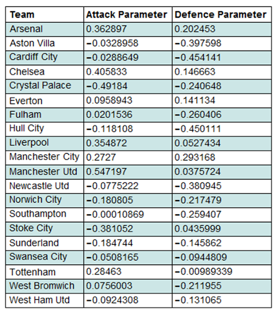
After compiling the evaluated parameters in a table, we were almost ready to start simulating games in the next season (2013/14). However we firstly needed to consider the team changes in the close season. At the end of the 2012/13 season the three bottom placed teams were relegated down to the division below, the Championship. These were Wigan Athletic, Reading and Queens Park Rangers. Their places in the Premier League in the 2013/14 season were taken by three teams promoted from the Championship. These were Cardiff City, Hull City and Crystal Palace. To reflect this in the model the relegated teams were swapped out for the promoted teams with the promoted teams inheriting the attack and defence parameters of the relegated teams.
teams1314=StringReplace[ptable1213[[All,1]],{"Wigan Athletic"->"Cardiff City","Reading"->"Hull City","QP Rangers"->"Crystal Palace"}];
ptable1314=SortBy[Transpose[{teams1314,attackcol,defencecol}],#[[1]]];
Grid[Prepend[%,{Style["Team",Bold],Style["Attack Parameter",Bold],Style["Defence Parameter",Bold]}],ItemStyle-> {"Text",FontSize->14},ItemSize->{Automatic,1.5},Alignment->{Left,Center},Frame->All,Background->{None,{{White,Lighter[Blend[{Blue,Green}],0.8`]}}}]
To carry out simulations we firstly needed to import results data from the 2013/14 season. This was extracted and cleaned in a similar way to the results data from the 2012/13 season.
data1314=Import["http://www.soccerstats.com/results.asp?league=england_2014","Data"];
Drop[Drop[Cases[data1314,{_,_,_,_,_},Infinity],None,{1,2}],None,{3}];
Drop[%,{1}];
Table[StringSplit[%[[i]],"-"],{i,1,n}];
resultsdata1314=Transpose[{StringTrim[%[[All,1,1]]],ToExpression[StringTrim[%[[All,2,1]]]],StringTrim[%[[All,1,2]]],ToExpression[StringTrim[%[[All,2,2]]]]}];
Export["results201314.xml",resultsdata1314];
Again we leave open the option to import the XML file instead in the case that this webpage also fails (see attached file) although it hasn't at the time of writing!
resultsdata1314=Import["results201314.xml"];
We now insert the gathered parameters for the strength of the home attack, away attack, home defence and away defence into each game of the 2013/14 season.
hattack=Flatten[Table[If[resultsdata1314[[j,1]]== ptable1314[[i,1]],ptable1314[[i,2]],##&[]],{j,1,n},{i,1,m}]];
aattack=Flatten[Table[If[resultsdata1314[[j,3]]== ptable1314[[i,1]],ptable1314[[i,2]],##&[]],{j,1,n},{i,1,m}]];
hdefence=Flatten[Table[If[resultsdata1314[[j,1]]== ptable1314[[i,1]],ptable1314[[i,3]],##&[]],{j,1,n},{i,1,m}]];
adefence=Flatten[Table[If[resultsdata1314[[j,3]]== ptable1314[[i,1]],ptable1314[[i,3]],##&[]],{j,1,n},{i,1,m}]];
fixtureparams=Transpose[{hattack,aattack,hdefence,adefence}];
Note that the actual score data has not been used whatsoever (no cheating here!) Next we calculate the expected goals scored for each team in every game of the season.
hgoalsfunction[x_,y_]:=Exp[x-y+homeadv]
agoalsfunction[x_,y_]:=Exp[x-y]
exphgoals=Table[hgoalsfunction[fixtureparams[[i,1]],fixtureparams[[i,4]]],{i,n}];
expagoals=Table[agoalsfunction[fixtureparams[[i,2]],fixtureparams[[i,3]]],{i,n}];
expresults=Transpose[{resultsdata1314[[All,1]],exphgoals,resultsdata1314[[All,3]],expagoals}];
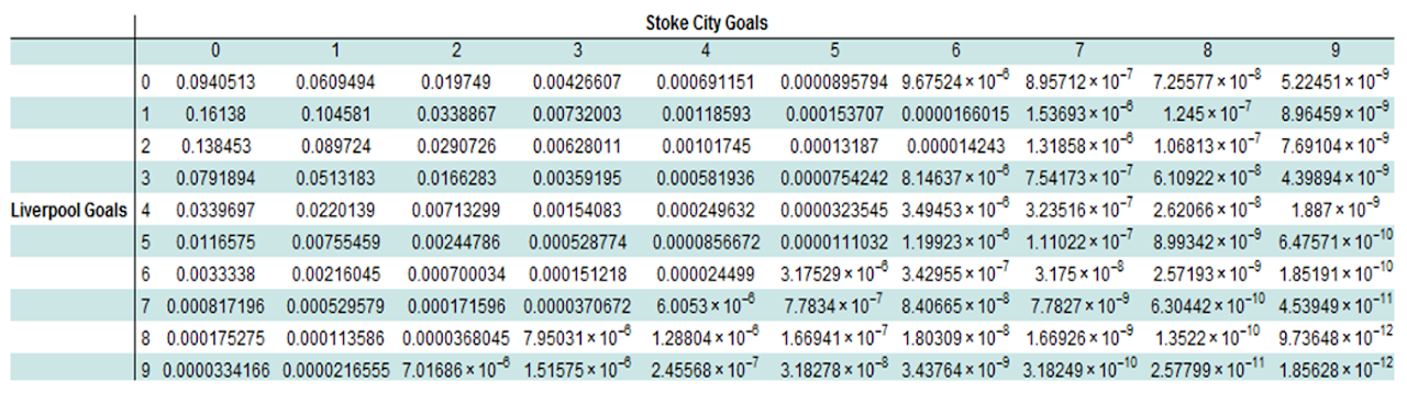
We are ready to simulate games. Before handling the task of simulating the entire season it was logical to first analyse one game only. We chose to dissect the first game of the 2013/14 season: Liverpool vs Stoke City. Using their respective parameters the goal expectancies were evaluated and Poisson distributed random integers with these expectations were computed.
livexpgoals=expresults[[1,2]];
stoexpgoals=expresults[[1,4]];
livscore=RandomInteger[PoissonDistribution[livexpgoals]];
stoscore=RandomInteger[PoissonDistribution[stoexpgoals]];
StringJoin["Liverpool ",ToString[livscore],"-",ToString[stoscore]," Stoke City"]

Now we analyse the probabilities of each score for this game, applying the probability density function for the Poisson distribution. Building a probability matrix allows us to get an overview of the output.
p[?_,x_]:=PDF[PoissonDistribution[?],x]
livprob=Table[p[livexpgoals,x],{x,0,10}];
stoprob=Table[p[stoexpgoals,x],{x,0,10}];
Table[livprob[[i]]*stoprob[[j]],{i,1,10},{j,1,10}];
Transpose[Prepend[Transpose[%],Range[0,9]]];
Prepend[%,{"",0,1,2,3,4,5,6,7,8,9}];
Prepend[%,{"","","","","",Style["Stoke City Goals",Bold],"","","","",""}];
Prepend[Transpose[%],{"","","","","","",Style["Liverpool Goals",Bold],"","","","",""}];
Grid[Transpose[%],ItemStyle->{"Text",FontSize->12},Dividers->{{False,True},{False,True}},Background->{None,{{White,Lighter[Blend[{Blue,Green}],0.8`]}}}]
A better visual representation of this is in the form of a 3-D plot.
DiscretePlot3D[((exphgoals[[1]]^x*Exp[-exphgoals[[1]]])/x!)*((expagoals[[1]]^y*Exp[-expagoals[[1]]])/y!),{x,0,6},{y,0,6},ExtentSize->Full,ImageSize->Large, ColorFunction->"Rainbow"]

This shows that the most probable outcome of this game was 1-0 to Liverpool with a likelihood of 16%; this just so happened to be the actual result of the game when it was played. The graphic also emphasises how unlikely high scoring games are with the probabilities being negligible.
This same procedure was then applied to every game of the season to obtain the expected goals for each team. This amounted to 760 calculations - two for each game.
homeexp=Flatten[Do[Sow[RandomInteger[PoissonDistribution[expresults[[i,2]]],1]],{i,1,n}]//Reap//Last//Last];
awayexp=Flatten[Do[Sow[RandomInteger[PoissonDistribution[expresults[[i,4]]],1]],{i,1,n}]//Reap//Last//Last];
poissonresults=Transpose[{resultsdata1314[[All,1]],homeexp,resultsdata1314[[All,3]],awayexp}];
To display these results in a more readable format, a league table was created which compiled all the results from the season. Points are awarded to teams as follows: 3 points for a win, 1 point for a draw and 0 points for a loss.
ConstantArray[0,{m,8}];
lge=Sort[Transpose[Prepend[Transpose[%],teams1314]]];
Do[Table[If[lge[[i,1]]==poissonresults[[j,1]]?lge[[i,1]]==poissonresults[[j,3]],lge[[i,2]]=lge[[i,2]]+1,##&[]],{i,1,m}]?Table[If[lge[[i,1]]==poissonresults[[j,1]],If[poissonresults[[j,2]]>poissonresults[[j,4]],lge[[i,3]]=lge[[i,3]]+1,##&[]],##&[]],{i,1,m}]?Table[If[lge[[i,1]]==poissonresults[[j,3]],If[poissonresults[[j,4]]>poissonresults[[j,2]],lge[[i,3]]=lge[[i,3]]+1,##&[]],##&[]],{i,1,m}]?Table[If[lge[[i,1]]==poissonresults[[j,1]],If[poissonresults[[j,2]]==poissonresults[[j,4]],lge[[i,4]]=lge[[i,4]]+1,##&[]],##&[]],{i,1,m}]?Table[If[lge[[i,1]]==poissonresults[[j,3]],If[poissonresults[[j,4]]==poissonresults[[j,2]],lge[[i,4]]=lge[[i,4]]+1,##&[]],##&[]],{i,1,m}]?Table[If[lge[[i,1]]==poissonresults[[j,1]],If[poissonresults[[j,2]]<poissonresults[[j,4]],lge[[i,5]]=lge[[i,5]]+1,##&[]],##&[]],{i,1,m}]?Table[If[lge[[i,1]]==poissonresults[[j,3]],If[poissonresults[[j,4]]<poissonresults[[j,2]],lge[[i,5]]=lge[[i,5]]+1,##&[]],##&[]],{i,1,m}]?Table[If[lge[[i,1]]==poissonresults[[j,1]],lge[[i,6]]=lge[[i,6]]+poissonresults[[j,2]],##&[]],{i,1,m}]?Table[If[lge[[i,1]]==poissonresults[[j,3]],lge[[i,6]]=lge[[i,6]]+poissonresults[[j,4]],##&[]],{i,1,m}]?Table[If[lge[[i,1]]==poissonresults[[j,1]],lge[[i,7]]=lge[[i,7]]+poissonresults[[j,4]],##&[]],{i,1,m}]?Table[If[lge[[i,1]]==poissonresults[[j,3]],lge[[i,7]]=lge[[i,7]]+poissonresults[[j,2]],##&[]],{i,1,20}],{j,1,n}]
Do[lge[[i,8]]=lge[[i,6]]-lge[[i,7]],{i,1,m}]
Do[lge[[i,9]]=3*lge[[i,3]]+1*lge[[i,4]],{i,1,m}]
singlesort=SortBy[lge,{-#[[9]],-#[[8]],-#[[7]]}&];
expleaguetable=Transpose[Prepend[Transpose[singlesort],Range[1,m]]];
Grid[Prepend[%,{"",Style["Team",Bold],Style["Pld",Bold],Style["W",Bold],Style["D",Bold],Style["L",Bold],Style["GF",Bold],Style["GA",Bold],Style["GD",Bold],Style["Pts",Bold]}],ItemStyle-> {"Text",FontSize->14},ItemSize->{Automatic,1.5},Alignment->{{Center,Left}},Frame->All,Background->{None,{{White,Lighter[Blend[{Blue,Green}],0.8`]}}}]
Having simulated one season, the next step was to emulate this over many seasons by attaching further loops. It was hypothesised that this would increase the accuracy level of the model. Several different numbers of simulations were tested, and it was found that beyond 100 iterations the accuracy level did not increase notably. This is a consequence of the shear number of calculations taking place. Since there are 380 games in a Premier League season, simulating 100 seasons requires 38,000 games to be computed, or 76,000 individual scores. This is a large enough number that increasing it further does not have an obvious effect on the accuracy level. Note that the notion of `accuracy level' is discussed in depth later.
s=100;
homeexp100=Table[RandomInteger[PoissonDistribution[expresults[[i,2]]],s],{i,1,n}];
awayexp100=Table[RandomInteger[PoissonDistribution[expresults[[i,4]]],s],{i,1,n}];
poissonresults100=Transpose[{resultsdata1314[[All,1]],homeexp100,resultsdata1314[[All,3]],awayexp100}];
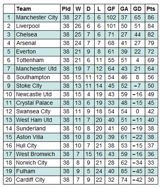
Again we construct a league table, this time taking the averages of all the statistics.
totallge=Sort[Transpose[Prepend[Transpose[ConstantArray[0,{m,8}]],teams1314]]];
lgepos={};
Monitor[Do[(simlge=Sort[Transpose[Prepend[Transpose[ConstantArray[0,{m,8}]],teams1314]]];
    Do[Table[If[simlge[[i,1]]==poissonresults100[[j,1]]?simlge[[i,1]]==poissonresults100[[j,3]],simlge[[i,2]]=simlge[[i,2]]+1,##&[]],{i,1,m}]?Table[If[simlge[[i,1]]==poissonresults100[[j,1]],If[poissonresults100[[j,2,x]]>poissonresults100[[j,4,x]],simlge[[i,3]]=simlge[[i,3]]+1,##&[]],##&[]],{i,1,m}]?Table[If[simlge[[i,1]]==poissonresults100[[j,3]],If[poissonresults100[[j,4,x]]>poissonresults100[[j,2,x]],simlge[[i,3]]=simlge[[i,3]]+1,##&[]],##&[]],{i,1,m}]?Table[If[simlge[[i,1]]==poissonresults100[[j,1]],If[poissonresults100[[j,2,x]]==poissonresults100[[j,4,x]],simlge[[i,4]]=simlge[[i,4]]+1,##&[]],##&[]],{i,1,m}]?Table[If[simlge[[i,1]]==poissonresults100[[j,3]],If[poissonresults100[[j,4,x]]==poissonresults100[[j,2,x]],simlge[[i,4]]=simlge[[i,4]]+1,##&[]],##&[]],{i,1,m}]?Table[If[simlge[[i,1]]==poissonresults100[[j,1]],If[poissonresults100[[j,2,x]]<poissonresults100[[j,4,x]],simlge[[i,5]]=simlge[[i,5]]+1,##&[]],##&[]],{i,1,m}]?Table[If[simlge[[i,1]]==poissonresults100[[j,3]],If[poissonresults100[[j,4,x]]<poissonresults100[[j,2,x]],simlge[[i,5]]=simlge[[i,5]]+1,##&[]],##&[]],{i,1,m}]?Table[If[simlge[[i,1]]==poissonresults100[[j,1]],simlge[[i,6]]=simlge[[i,6]]+poissonresults100[[j,2,x]],##&[]],{i,1,20}]?Table[If[simlge[[i,1]]==poissonresults100[[j,3]],simlge[[i,6]]=simlge[[i,6]]+poissonresults100[[j,4,x]],##&[]],{i,1,m}]?Table[If[simlge[[i,1]]==poissonresults100[[j,1]],simlge[[i,7]]=simlge[[i,7]]+poissonresults100[[j,4,x]],##&[]],{i,1,m}]?Table[If[simlge[[i,1]]==poissonresults100[[j,3]],simlge[[i,7]]=simlge[[i,7]]+poissonresults100[[j,2,x]],##&[]],{i,1,m}]?Do[simlge[[i,8]]=1*simlge[[i,6]]-simlge[[i,7]],{i,1,m}]\[And]
      Do[simlge[[i,9]]=3*simlge[[i,3]]+1*simlge[[i,4]],{i,1,m}],{j,1,n}])\[And]
   (totallge[[All,2;;9]]=totallge[[All,2;;9]]+simlge[[All,2;;9]])\[And]
   (sorttmp=SortBy[simlge,{-#[[9]],-#[[8]],-#[[7]]}&])\[And]
   (AppendTo[lgepos,sorttmp[[All,1]]]),
  {x,1,s}],ProgressIndicator[x/s]]
simsort=SortBy[totallge,{-#[[9]],-#[[8]],-#[[7]]}&];
simexpleague=Transpose[Prepend[Transpose[simsort],Range[1,m]]];
Insert[Grid[Prepend[%,{"",Style["Team",Bold],Style["Pld",Bold],Style["W",Bold],Style["D",Bold],Style["L",Bold],Style["GF",Bold],Style["GA",Bold],Style["GD",Bold],Style["Pts",Bold]}],Alignment->Left,Frame->All],{Background->{None,{{White,Lighter[Blend[{Blue,Green}],0.8`]}}},Dividers->Black,Frame->True,Spacings->{2,{2,{0.7`},2}}},2];
Transpose[(Table[simexpleague[[All,c]],{c,3,10}])/s//N];
Transpose[Prepend[Transpose[%],simexpleague[[All,2]]]];
Transpose[Prepend[Transpose[%],Range[1,m]]];
Grid[Prepend[%,{"",Style["Team",Bold],Style["Pld",Bold],Style["W",Bold],Style["D",Bold],Style["L",Bold],Style["GF",Bold],Style["GA",Bold],Style["GD",Bold],Style["Pts",Bold]}],ItemStyle-> {"Text",FontSize->14},ItemSize->{Automatic,1.5},Alignment->{{Center,Left}},Frame->All,Background->{None,{{White,Lighter[Blend[{Blue,Green}],0.8`]}}}]

Using data accrued in the above code, we can find out which teams won the league title over the 100 seasons, and how many times they did so.
Flatten[SortBy[Tally[lgepos[[All,1]]],-#[[2]]&]];
BarChart[Take[%,{2,-1,2}],ChartStyle->"DarkRainbow",AxesLabel->{Style["Team",FontSize->10],Style["Occurrences",FontSize->10]},ChartLegends->Take[%,{1,-1,2}],ImageSize->Large]

More generally, we can construct a table which shows how many times each team finished in each league position over the 100 seasons.
allpos=Table[Table[Total[Table[If[lgepos[[All,k]][[i]]==ptable1314[[j,1]],1,0],{i,1,s}]],{k,1,m}],{j,1,m}];
Transpose[Prepend[Transpose[allpos],Style[#,Bold]&/@ptable1314[[All,1]]]];
Grid[Prepend[%,{"",Style["1",Bold],Style["2",Bold],Style["3",Bold],Style["4",Bold],Style["5",Bold],Style["6",Bold],Style["7",Bold],Style["8",Bold],Style["9",Bold],Style["10",Bold],Style["11",Bold],Style["12",Bold],Style["13",Bold],Style["14",Bold],Style["15",Bold],Style["16",Bold],Style["17",Bold],Style["18",Bold],Style["19",Bold],Style["20",Bold]}],ItemStyle-> {"Text",FontSize->14},ItemSize->{Automatic,1.5},Alignment->{{Left,Center}},Frame->All,Background->{None,{{White,Lighter[Blend[{Blue,Green}],0.8`]}}}]

A more visual representation of sections of this data is via a bar chart.
BarChart[allpos[[6]],ChartStyle->"DarkRainbow",ChartLabels->Range[1,m],AxesLabel->{Style["Position",FontSize->10],Style["Occurrences",FontSize->10]},ImageSize->Large]

Here we have the number of times Everton finished in each league position over the 100 seasons. This graph indicates that Everton are likely to finish in the top half, and may even have a chance of finishing in the top four, thus qualifying for Europe. It also shows that Everton are almost certainly not going to finish in the bottom three and be relegated. Lastly, we can compare the performance of teams using a paired bar chart.
PairedBarChart[allpos[[6]],allpos[[17]],ChartStyle->"DarkRainbow",ChartLabels->Range[1,m],AxesLabel->{Style["Occurrences",FontSize->10],Style["Position",FontSize->10]},ImageSize->Large]

Here the left side again shows Evertons league positions over the 100 seasons, while the right side shows the same data for Swansea City. Although both teams are likely to finish in the top half, we can conclude that Everton are generally the better team - Swansea have many more bottom half finishes, and may even have a chance of finishing in the bottom three and being relegated.
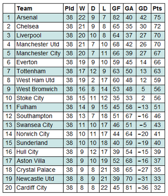
To determine the accuracy of the model, we undertook some tests to compare the outcome of both the single simulation and the 100 simulations to the actual outcome of the 2013/14 season. Firstly, we construct the actual league table for the 2013/14 season using the results data from earlier.
ConstantArray[0,{m,8}];
actual=Sort[Transpose[Prepend[Transpose[%],teams1314]]];
Do[Table[If[actual[[i,1]]==resultsdata1314[[j,1]]?actual[[i,1]]==resultsdata1314[[j,3]],actual[[i,2]]=actual[[i,2]]+1,##&[]],{i,1,m}]?Table[If[actual[[i,1]]==resultsdata1314[[j,1]],If[resultsdata1314[[j,2]]>resultsdata1314[[j,4]],actual[[i,3]]=actual[[i,3]]+1,##&[]],##&[]],{i,1,m}]?Table[If[actual[[i,1]]==resultsdata1314[[j,3]],If[resultsdata1314[[j,4]]>resultsdata1314[[j,2]],actual[[i,3]]=actual[[i,3]]+1,##&[]],##&[]],{i,1,m}]?Table[If[actual[[i,1]]==resultsdata1314[[j,1]],If[resultsdata1314[[j,2]]==resultsdata1314[[j,4]],actual[[i,4]]=actual[[i,4]]+1,##&[]],##&[]],{i,1,m}]?Table[If[actual[[i,1]]==resultsdata1314[[j,3]],If[resultsdata1314[[j,4]]==resultsdata1314[[j,2]],actual[[i,4]]=actual[[i,4]]+1,##&[]],##&[]],{i,1,m}]?Table[If[actual[[i,1]]==resultsdata1314[[j,1]],If[resultsdata1314[[j,2]]<resultsdata1314[[j,4]],actual[[i,5]]=actual[[i,5]]+1,##&[]],##&[]],{i,1,m}]?Table[If[actual[[i,1]]==resultsdata1314[[j,3]],If[resultsdata1314[[j,4]]<resultsdata1314[[j,2]],actual[[i,5]]=actual[[i,5]]+1,##&[]],##&[]],{i,1,m}]?Table[If[actual[[i,1]]==resultsdata1314[[j,1]],actual[[i,6]]=actual[[i,6]]+resultsdata1314[[j,2]],##&[]],{i,1,m}]?Table[If[actual[[i,1]]==resultsdata1314[[j,3]],actual[[i,6]]=actual[[i,6]]+resultsdata1314[[j,4]],##&[]],{i,1,m}]?Table[If[actual[[i,1]]==resultsdata1314[[j,1]],actual[[i,7]]=actual[[i,7]]+resultsdata1314[[j,4]],##&[]],{i,1,m}]?Table[If[actual[[i,1]]==resultsdata1314[[j,3]],actual[[i,7]]=actual[[i,7]]+resultsdata1314[[j,2]],##&[]],{i,1,m}],{j,1,n}]
Do[actual[[i,8]]=actual[[i,6]]-actual[[i,7]],{i,1,m}]
Do[actual[[i,9]]=3*actual[[i,3]]+1*actual[[i,4]],{i,1,m}]
SortBy[actual,{-#[[9]],-#[[8]],-#[[7]]}&];
actuallge=Transpose[Prepend[Transpose[%],Range[1,m]]];
Grid[Prepend[%,{"",Style["Team",Bold],Style["Pld",Bold],Style["W",Bold],Style["D",Bold],Style["L",Bold],Style["GF",Bold],Style["GA",Bold],Style["GD",Bold],Style["Pts",Bold]}],ItemStyle-> {"Text",FontSize->14},ItemSize->{Automatic,1.5},Alignment->{{Center,Left}},Frame->All,Background->{None,{{White,Lighter[Blend[{Blue,Green}],0.8`]}}}]
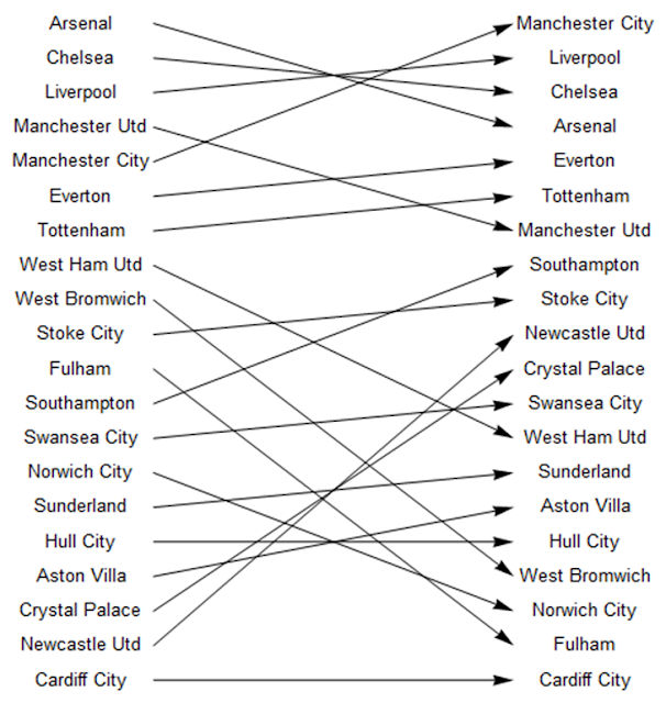
The first check involved producing diagrams which compared the league position of each team in the two simulations to their actual league position. Firstly the single simulation:
sim1teams=singlesort[[All,1]];
actualteams=actuallge[[All,2]];
Do[Do[If[sim1teams[[i]]==actualteams[[j]],x[i]=Graphics[Arrow[{{0,21-i},{10,21-j}}],##&[]]],{i,1,20}],{j,1,20}]
vert=Graphics[Table[Text[sim1teams[[i]],{-2,21-i},{0,0}],{i,1,20}]];
vert2=Graphics[Table[Text[actualteams[[i]],{12,21-i},{0,0}],{i,1,20}]];
Show[vert,vert2,Table[x[i],{i,1,20}]]
And then the 100 simulations:
simteams=simsort[[All,1]];
actualteams=actuallge[[All,2]];
Do[Do[If[simteams[[i]]==actualteams[[j]],x[i]=Graphics[Arrow[{{0,21-i},{10,21-j}}],##&[]]],{i,1,20}],{j,1,20}]
vertical=Graphics[Table[Text[simteams[[i]],{-2,21-i},{0,0}],{i,1,20}]];
vertical2=Graphics[Table[Text[actualteams[[i]],{12,21-i},{0,0}],{i,1,20}]];
Show[vertical,vertical2,Table[x[i],{i,1,20}]]
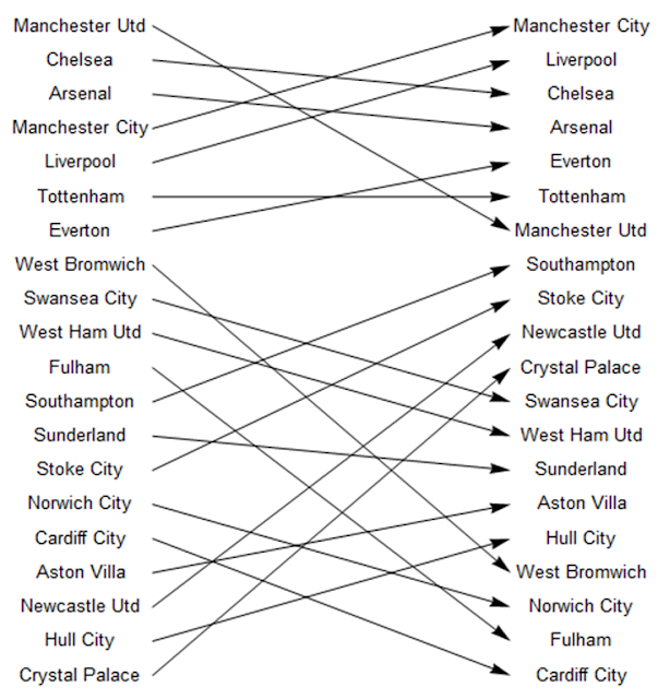
These indicated a low level of accuracy with regard to league positions. Nonetheless, a consequent observation was that there appear to be two mini-leagues within the Premier League - the top seven teams and the rest. With qualification for European competitions often awarded to the teams finishing in the first seven positions, and the financial revenue this brings to these clubs, it may be that this allows these teams to maintain greater stability and consolidate these positions higher up the league table.
A more thorough test of the accuracy of the model involved comparing both the outcomes (home win, away win or draw) and scores on a game-by-game basis.
correctoutcome=0;
correctoutcome100=0;
correctscore=0;
correctscore100=0;
avghome=Table[Mean[homeexp100[[i]]],{i,1,n}]//N;
avgaway=Table[Mean[awayexp100[[i]]],{i,1,n}]//N;
Do[If[homeexp[[i]]>awayexp[[i]]?resultsdata1314[[i,2]]>resultsdata1314[[i,4]],correctoutcome=correctoutcome+1,If[homeexp[[i]]<awayexp[[i]]?resultsdata1314[[i,2]]<resultsdata1314[[i,4]],correctoutcome=correctoutcome+1,If[homeexp[[i]]==awayexp[[i]]?resultsdata1314[[i,2]]==resultsdata1314[[i,4]],correctoutcome=correctoutcome+1,##&[]]]],{i,1,n}]
Do[If[homeexp[[i]]==resultsdata1314[[i,2]]?awayexp[[i]]==resultsdata1314[[i,4]],correctscore=correctscore+1,##&[]],{i,1,n}]
Do[If[avghome[[i]]>avgaway[[i]]?resultsdata1314[[i,2]]>resultsdata1314[[i,4]],correctoutcome100=correctoutcome100+1,If[avghome[[i]]<avgaway[[i]]?resultsdata1314[[i,2]]<resultsdata1314[[i,4]],correctoutcome100=correctoutcome100+1,If[avghome[[i]]==avgaway[[i]]?resultsdata1314[[i,2]]==resultsdata1314[[i,4]],correctoutcome100=correctoutcome100+1,##&[]]]],{i,1,n}]
Do[If[Round[avghome[[i]]]==resultsdata1314[[i,2]]?Round[avgaway[[i]]]==resultsdata1314[[i,4]],correctscore100=correctscore100+1,##&[]],{i,1,n}]
{correctoutcome,correctscore,correctoutcome100,correctscore100}*100/n"%"//N;
Grid[Transpose[{{Style["One simulation",Bold],SpanFromAbove,Style["100 simulations",Bold],SpanFromAbove},{"Outcome","Score","Outcome","Score"},%}],Frame->All,Alignment->{Left,Center},ItemStyle-> {"Text",FontSize->14},ItemSize->{Automatic,1.5}]
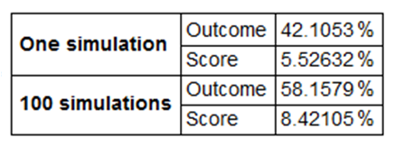
In one particular case, the model predicted the correct outcome in approximately 42% of games in the single simulation and 58% of games in the 100 simulations. In terms of scores, the model was correct in approximately 6% of games in the single simulation and 8% of games in the 100 simulations. As was previously hypothesised, the 100 simulations were much more accurate than the single simulation.
In conclusion, the model highlights that it is possible to predict the outcome of a football game with some degree of accuracy, but predicting perfect scores is much more difficult. However, there is much refinement could be made to the model to improve the accuracy levels, not least with the addition of more parameters.
 Attachments:


