We present alternative methods for Incremental Risk Calculation which is one of the key pillars of new capital regime for financial institutions under the comprehensive review of the Trading Book – known as Basel 2.5. The primary analytical tool is the Copula method which enables efficient mixing of marginals into a full-scale multivariate distributions. We test various distributional assumptions and find significant variations in the model measure when different assumptions about risk dynamics are used.

Objectives

We will review alternative approaches to IRC modelling where we explore the full power and flexibility of Wolfram Finance Platform - both in symbolic and numerical domains. Our modelling basis resides on hazard rate process, Bernoulli event and their extensions to the multivariate setting in the portfolio context where we employ copulas.

We show that this approach is quick and can be extended in various dimensions to accommodate various institution-specific constraints.

IRC - Background

IRC is an integral component of the banks' capital regime and therefore attracts due attention from both regulatory practice and financial professionals who require accurate and robust methods for calculation of this measure

• IRC - the new risk measure (since 2009) as a part of comprehensive review of Trading Book under Basel 2.5.
• The general consensus relies on the notation of undercapitalisation and to some extent unpreparedness to withstand severe financial shocks. Banks have to enhance their capital position

Why IRC?

One of the most critical weaknesses of the pre-crisis capital framework was the inability of Value-at-Risk (VaR) models to capture asset value deterioration due to credit risk migration.

• Historical observations => massive losses occurred not due to the actual issuers' defaults, but due to credit risk explosion in financial assets (primality bonds and credit default swaps) held on the trading books required to be marked-to-market
• In essence, the losses were generated by significant widening of credit spreads and rating deterioration
• In this respect IRC is a regulatory response to the above problem and its primary objective is to address the VaR limitations in spread migration domain

Capital regime and IRC

• Capital requirements under Base II:

$RC = (MM+F) VaR + VaR(S)$

where: MM= model multiplier >= 3 , 0<=F<1 is the back-testing excess factor , VaR = the 10-day 99% loss , VaR(S) = specific VaR

• The risk formula has been significantly enhanced in the Basel 2.5 framework to include:

$RC (New) =(MM_c+F)VaR + (MM_s+F)StVaR + IRC +Max[CRM, Floor] + SC$

where: StVaR = Stresses VaR with its own factor , IRC = Incremental Risk Charge , CRM = incremental charge for correlation trading books s.t. minimum prescribed floor level , SC = securitised positions specific charge

• As we can see, the new risk capital calculation is more advanced and comprehensive:

  • Addresses each individual risk factors separately
  • Financial institutions subject to regulatory control are required to calculate the IRC at least weekly with 99.9% confidence with one year capital horizon

• IRC goes beyond VaR in two aspects:

  • (i) confidence interval extends "deeper" into the tail of the loss distribution with higher confidence limit[99.9%]
  • (ii) capital horizon is set to 1-year, as opposed to 10-day market risk VaR calculation
• Given the length of capital horizon, regulator allows shorter "liquidity" time frames (min of 3 months) for portfolio re-balancing, however the "constant level of risk" must be preserved

IRC Methodologies

• Given the scope and definition, the measure can be calculated in a number of ways. The most frequently used are: Rating-based approach with rating migration profile

• Credit spread modelling approach with evolutionary default probabilities

• Mixture methods where both approaches are combined into coherent modelling framework

Our preferred choice:

• Direct approach to credit spread that contains all relevant information about the creditworthiness of each issuer.

• With defined recovery rate , the spread determines the default probability for each issuer in the portfolio that will drive and affect the loss distribution

• We will employ standard credit spread modelling approaches for clarity and consistency purposes and demonstrate the ease of the implementation of the proposed solution.

Defining components of the IRC methods

When dealing with large portfolio of credit-sensitive instruments, it may be advisable to break down the entire set of assets into smaller "clusters"with some common features

• Ratings - external or internal - have been for some time a preferred choice for asset grouping with similar credit-quality
  • This is because rating clusters enable the treatment of the subset with consistent set of parameters

We assume constant rates and also the notion that credit spread and recovery information exists for each issuer in the cluster. We define the following measures:

• Hazard rate: $ h=Spread/((1-R)T) $

• Survival probability: $Q=Exp[-h*T]$

• Cumulative default probability: $F = 1 - Q = 1 - Exp[-h*T]$

• If we assume that the default represented though the hazard rate is a Bernoulli event with parameter h, we obtain the volatility of the hazard rate as:

  • $vol= Sqrt[h(1-h)] $

Knowing the market-implied hazard rate and its volatility enables us to build distributional models for hazard rate process that will drive the future losses in the portfolio due to credit quality deterioration

• This represents the alternative to more traditional rating migration approach and here we simply assume that the hazard rate evolution through time is a stochastic process with a given stationary distribution H(T) from which we can compute quantiles at a prescribed confidence level of 99.9%

• Risk-adjusted maturity: $T_r=T*Q$

Portfolio credit risk

What is special about the portfolio of credit-sensitive assets?

• It is similar to individual assets, however beside credit exposure we need to include dependency structure - i.e. the tendency how individual assets react together. Dependency is critically important as it affects the likelihood of joint events such as portfolio loss

  • The higher the probability of the joint deterioration of creditworthiness, the bigger the portfolio loss

• Probabilistically, the credit portfolio = collection of individual assets (random variables) [Pi]={Subscript[X, 1],Subscript[X, 2],...Subscript[X, n],}

  • Our primary tool for the analysis => multivariate distributions

• Preferred choice for the study is dependency structure is the Copulae approach

• Correlation is probably the best known measure of dependency in finance.

  • Although not necessarily true, the association of correlation with dependency is strongly embedded in the mindset of financial professionals

  • For the ease of exposition, we will select copulas that explicitly take correlation matrix as an input

• In the credit portfolio context we need to be careful about which correlation to use. Since our building block is the hazard rate, we essentially need the correlation of hazard rates, which, however, is not directly observable in the market

  • The hazard rate correlation is defined as

  • The only difficultly in this formula is the calculation of joint expectation. Bi-normal copula can be easily applied in this setting and correlation can be obtained from this joint distribution. This is available in Wolfram Finance Platform (WFP) so the hazard rate correlation above can be directly obtained from the Bi normal copula with Bernoulli marginals ${h_1, h_2}$ and asset correlation $\rho$.

    BerCop = CopulaDistribution[{"Binormal", \[Rho]}, {BernoulliDistribution[h1], BernoulliDistribution[h2]}];
    Correlation[BerCop, 1, 2]
    

  

      % /. {\[Rho] -> 0.3, h1 -> 0.03, h2 -> 0.05}
  

0.0867005

• Note that the hazard rate correlation (8.6%) is much lower number than the asset correlation (30%) used in the Bi-normal copula. This is supported by empirical evidence

To complete the credit portfolio setup, we further define:

• Weighted-average risky duration:

where w = normalised weight vector of each asset in the cluster

• Weighted-average hazard rate:

• Clustered portfolio volatility:

Hazard rate process

Reduction of clustered portfolio dimensionality into single variable moments is a practical step for multi-cluster modelling. We can model the hazard rate evolution through some known Ito stochastic processes, calculate their moments and then parametrise distributional assumptions. The following models can be applied here:

• 
• Each process represents 'single' cluster risk evolution. We combined clusters through copulas, define their joint distributions and obtain their quantiles. Quantiles then lead to the 'cluster loss' measure
• IRC is finally the sum of all individual cluster losses.

WFP / Mathematica implementation

• WFP - ideal for this task:

  • Offers computational efficiency

  • Provides required functional interfaces and great visualisation tools

• We assume:

  • 5 rating categories in the portfolio: A,B,C,D,E

  • Same amount per cluster = 100 mil

  • Demonstrate the implementation with portfolio A:

• 10 positions with maturity from 1 to 10 years

• CDS spreads vary between 100~250 bp

   - Each position is represented by its weight in the range [0,1]
  

.

mat = RandomSample[Range[0.75, 10, 0.1], 10]
cds = RandomSample[Range[0.01, 0.025, 0.001], 10]
wr = RandomSample[Range[0, 1, 0.01], 10];  w = Normalize[wr, Total]

{3.65, 1.75, 6.35, 8.55, 2.95, 6.15, 4.95, 3.85, 5.15, 1.15}

{0.018, 0.015, 0.02, 0.016, 0.023, 0.022, 0.021, 0.019, 0.014, 0.01}

{0.191083, 0.106157, 0.11465, 0.201699, 0.0127389, 0.00424628, 0.0339703, 0.161359, 0.0997877, 0.07431}

• We assume 35% recovery for each asset in the cluster and from there we calculate the hazard rate, cumulative default probability and the hazard rate volatility

  h = cds/((1 - 0.35) mat)
  F = 1 - Exp[-h*mat]
  rdur = mat*Exp[-h*mat]
  vol = Sqrt[h (1 - h)]
  

{0.00758693, 0.0131868, 0.00484555, 0.00287899, 0.0119948, 0.00550344, 0.00652681, 0.00759241, 0.00418223, 0.0133779}

{0.0273124, 0.0228127, 0.0303007, 0.0243149, 0.0347659, 0.0332798, 0.0317914, 0.0288077, 0.0213082, 0.0152669}

{3.55031, 1.71008, 6.15759, 8.34211, 2.84744, 5.94533, 4.79263, 3.73909, 5.04026, 1.13244}

{0.086772, 0.114074, 0.0694411, 0.0535789, 0.108862, 0.0739808, 0.0805246, 0.086803, 0.0645348, 0.114887}

• We build the following (low-level) correlation structure:

  CM[n_] := 
   Module[{tb, ms}, 
    tb = Table[
      If[i == j, 1/2, If[j > i, RandomReal[{0, 0.15}], 0]], {i, n}, {j, 
       n}];
    ms = tb + Transpose[tb]]
  CM[10] // MatrixForm
  

Obtaining cluster characteristics

We compute the following measures

• Risk-adjusted duration

• Weighted-average hazard rate

• Weighted hazard rate volatility

  wvol = w*vol
  cdur = Total[w*rdur]
  chmean = Total[w*rdur*h]/cdur
  cvol = Sqrt[wvol.CM[10].wvol]
  

{0.0165806, 0.0121098, 0.0079614, 0.0108068, 0.00138678, 0.000314143, 0.00273544, 0.0140064, 0.00643977, 0.00853723} 4.66327 0.0054152 0.0367442

This shows that the our Rating A Cluster with 100 mil of assets has risky duration of 4.66 years, risk-adjusted hazard rate of 54 bp and hazard rate volatility of 3.67%.

• We skip the repeat of the above for each cluster and simply assume the following measures:

• Duration per cluster:

  tdur = Table[
    If[i < 1, cdur, cdur*Exp[RandomReal[{0.1, 0.35}]]], {i, 0, 4}]
  

{4.66327, 5.83364, 5.59038, 6.52077, 5.42679}

• Hazard rate:

  thmean = Table[
    If[i < 1, chmean, chmean*Exp[RandomReal[{0.1, 0.25}]]], {i, 0, 4}]
  

{0.0054152, 0.00625678, 0.00641638, 0.00653013, 0.00671054}

• Volatility:

  tvol = Table[If[i < 1, cvol, cvol*Exp[RandomReal[{0.05, 0.15}]]], {i, 0, 4}]
  

{0.0367442, 0.0415985, 0.0397301, 0.0419299, 0.0388844}

• Inter-cluster correlation matrix:

  clcorrel = ({
      {1, 0.21, 0.2, 0.23, 0.16},
      {0.21, 1, 0.18, 0.16, 0.25},
      {0.2, 0.18, 1, 0.19, 0.29},
      {0.23, 0.16, 0.19, 1, 0.17},
      {0.16, 0.25, 0.29, 0.17, 1}
     } );
  

  • from which we build the Covariance matrix:

    CovarMatrix[cm_, vols_] := 
     Module[{n, fms}, n = Length[vols]; 
      fms = Table[cm[[i, j]]*vols[[i]]*vols[[j]], {i, n}, {j, n}]]
    clcovar = CovarMatrix[clcorrel, tvol];
    CovarMatrix[clcorrel, tvol] // MatrixForm
    

  

Defining Copulae

Depending on the hazard rate process specification, we get the following calibration output for the forward hazard rate setting - in terms of mean and volatility of the stationary process:

• Normal process:

  ito = ItoProcess[{\[Mu], \[Sigma]}, {x, x0}, t];
  {Mean[ito[t]], StandardDeviation[ito[t]]}
  

• Mean-reverting normal process:

  ito = ItoProcess[{\[CurlyTheta] (\[Mu] - x), \[Sigma]}, {x, x0}, t];
  {Mean[ito[t]], StandardDeviation[ito[t]]} // Simplify
  

• Log-Normal process:

  ito = ItoProcess[{\[Mu]*x, \[Sigma]*x}, {x, x0}, t];
  {Mean[ito[t]], StandardDeviation[ito[t]]} // Simplify
  

• Square-root diffusion process:

  ito = ItoProcess[{\[CurlyTheta] (\[Mu] - x[t]), \[Sigma]*Sqrt[x[t]]}, {x, x0}, t];
  {Mean[ito[t]], StandardDeviation[ito[t]]} // Simplify
  

If we know the drift and diffusion parameters, the terminal forward rates can be easily obtained form the above formulas

• Consider the simplest case - the Normal process and assume that t=1 and we set the process drift $\mu=0$. This will lead to the following model calibration: mean = cluster's weighted-average hazard rate and vol = cluster's volatility.

  ito = ItoProcess[{\[Mu], \[Sigma]}, {x, x0}, t];
  {Mean[ito[t]], StandardDeviation[ito[t]]} /. {t -> 1, \[Mu] -> 0} // TraditionalForm
  

• If the aim is to preserve full correlation structure of all rating classes, we have two copula choices (i) Gaussian and (ii) StudentT:
  • Gaussian:
  • StudentT:

Gaussian Copulae model

Let's recall the basis parameters:

thmean
tvol

{0.0054152, 0.00625678, 0.00641638, 0.00653013, 0.00671054}

{0.0367442, 0.0415985, 0.0397301, 0.0419299, 0.0388844}

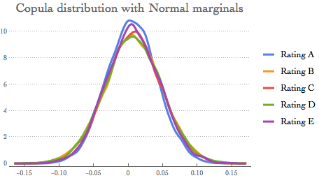
• GC with Normal marginals - 99.9% quantiles

  cdNorm = CopulaDistribution[{"Multinormal", clcovar}, 
     Table[NormalDistribution[thmean[[i]], tvol[[i]]], {i, 1, 5}]];
  rsample = RandomVariate[cdNorm, 10^4];
  ircNormhr = Quantile[rsample, 0.999]
  

{0.115322, 0.128352, 0.126666, 0.13725, 0.131207}

• Graphical representation

  SmoothHistogram[{rsample[[All, 1]], rsample[[All, 2]], 
    rsample[[All, 3]], rsample[[All, 4]], 
    rsample[[All, 5]]}, Automatic, "PDF", 
   PlotLabel -> Style["Copula distribution with Normal marginals", 18], 
   PlotTheme -> "Business", 
   PlotLegends -> {"Rating A", "Rating B", "Rating C", "Rating D", "Rating E"}]
  

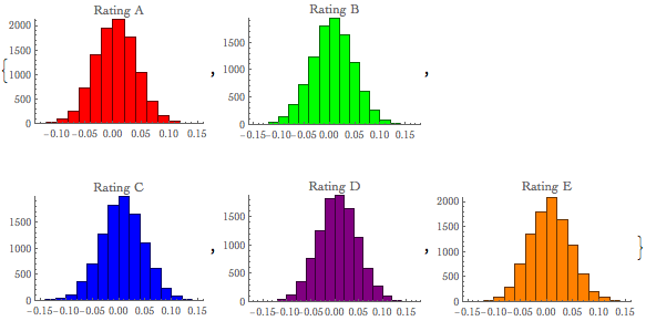
• We can also easily visualise each cluster with histograms

  {Histogram[Style[rsample[[All, 1]], Red], PlotLabel -> "Rating A"], 
   Histogram[Style[rsample[[All, 2]], Green], PlotLabel -> "Rating B"], 
   Histogram[Style[rsample[[All, 3]], Blue], PlotLabel -> "Rating C"], 
   Histogram[Style[rsample[[All, 4]], Purple], PlotLabel -> "Rating D"], 
   Histogram[Style[rsample[[All, 5]], Orange], PlotLabel -> "Rating E"]}
  

Mixture copulae models

We use the Gaussian Copulae with different marginals to create 'mixture' dynamics

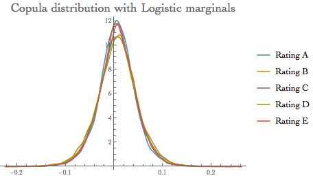
• Logistic marginals model: Logistic model is one of the alternatives to the Normal copula model where we draw marginals from Logistic probability distributions. Parametrisation is done through moment matching where Mean [XYZ] ==$ \eta$ && Variance[XYZ]==$\sigma^2$

Recall: the PDF for value x in a logistic model is proportional to $E^(-(x-\mu)/\beta)/(1+E^(-(x-\mu)/\beta))$

dsoln1 = Refine[Solve[{Mean[LogisticDistribution[a, b]] == \[Eta], 
     Variance[LogisticDistribution[a, b]] == \[Sigma]^2}, {a, b}, Reals], {\[Sigma] > 0}];

calcmean = Table[dsoln1[[1, 1, 2]] /. {\[Eta] -> thmean[[i]], \[Sigma] -> tvol[[i]]}, {i, 1, 5}];

calcvol = Table[dsoln1[[2, 2, 2]] /. {\[Eta] -> thmean[[i]], \[Sigma] -> tvol[[i]]}, {i, 1, 5}];

cdLogistic = CopulaDistribution[{"Multinormal", clcovar}, Table[LogisticDistribution[calcmean[[i]], calcvol[[i]]], {i, 1, 5}]];

rsample = RandomVariate[cdLogistic, 10^4];

ircLogistichr = Quantile[rsample, 0.999]

{0.137919, 0.173553, 0.172077, 0.166075, 0.155967}

• Visualising the model output:

  SmoothHistogram[{rsample[[All, 1]], rsample[[All, 2]], rsample[[All, 3]], rsample[[All, 4]], rsample[[All, 5]]},
   Automatic, "PDF", 
   PlotLabel -> Style["Copula distribution with Logistic marginals", 18], 
   PlotLegends -> {"Rating A", "Rating B", "Rating C", "Rating D", "Rating E"}]
  

• Laplace marginals model

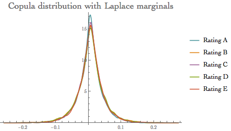
The Laplace distribution gives the distribution of the difference between two independent random variables with identical exponential distributions with PDF:

PDF[LaplaceDistribution[\[Mu], \[Beta]], x]

dsoln = Refine[
   Solve[{Mean[LaplaceDistribution[a, b]] == \[Eta], 
     Variance[LaplaceDistribution[a, b]] == \[Sigma]^2}, {a, b}, 
    Reals], {\[Sigma] > 0}];
calcmean = 
  Table[dsoln[[1, 1, 
     2]] /. {\[Eta] -> thmean[[i]], \[Sigma] -> tvol[[i]]}, {i, 1, 5}];
calcvol = 
  Table[dsoln[[2, 2, 
     2]] /. {\[Eta] -> thmean[[i]], \[Sigma] -> tvol[[i]]}, {i, 1, 5}];
cdLaplace = 
  CopulaDistribution[{"Multinormal", clcovar}, 
   Table[LaplaceDistribution[calcmean[[i]], calcvol[[i]]], {i, 1, 5}]];
rsample = RandomVariate[cdLaplace, 10^4];
ircLaplacehr = Quantile[rsample, 0.999]

{0.147783, 0.19349, 0.171785, 0.171115, 0.172867}

SmoothHistogram[{rsample[[All, 1]], rsample[[All, 2]], 
  rsample[[All, 3]], rsample[[All, 4]], 
  rsample[[All, 5]]}, Automatic, "PDF", 
 PlotLabel -> Style["Copula distribution with Laplace marginals", 18],
  PlotRange -> All, 
 PlotLegends -> {"Rating A", "Rating B", "Rating C", "Rating D",  "Rating E"}]

GC with Stable family marginals

• Stable marginals model

A stable distribution is defined in terms of its characteristic function $\phi(t)$ , which satisfies a functional equation where for any a and b there exist c and h such that $\phi(a t) \phi(b t)=\phi(c t) exp(I h t)$

dsoln = Refine[Solve[{Mean[StableDistribution[1, 2, 1, a, b]] == \[Eta], 
     Variance[StableDistribution[1, 2, 1, a, b]] == \[Sigma]^2}, {a, b}, Reals], {\[Sigma] > 0}];

calcmean = Table[dsoln[[1, 1, 2]] /. {\[Eta] -> thmean[[i]], \[Sigma] -> tvol[[i]]}, {i, 1, 5}];

calcvol = Table[dsoln[[2, 2,  2]] /. {\[Eta] -> thmean[[i]], \[Sigma] -> tvol[[i]]}, {i, 1, 5}];

cdStable = CopulaDistribution[{"Multinormal", clcovar}, 
   Table[StableDistribution[1, 2, 1, calcmean[[i]], calcvol[[i]]], {i,1, 5}]];

rsample = RandomVariate[cdStable, 10^4];

ircStablehr = Quantile[rsample, 0.999]

{0.117744, 0.131838, 0.130584, 0.132754, 0.127134}

{SmoothHistogram[{rsample[[All, 1]], rsample[[All, 2]], 
   rsample[[All, 3]], rsample[[All, 4]], rsample[[All, 5]]}, 
  Automatic, "PDF", 
  PlotLabel -> Style["Copula distribution with Stable marginals", 18],
   PlotLegends -> {"Rating A", "Rating B", "Rating C", "Rating D", 
    "Rating E"}, PlotTheme -> "Business", ImageSize -> 300], 
 SmoothHistogram[{rsample[[All, 1]], rsample[[All, 2]], 
   rsample[[All, 3]], rsample[[All, 4]], rsample[[All, 5]]}, 
  Automatic, "PDF", 
  PlotLabel -> Style["Tail focus: GC with Stable marginals", 16], 
  PlotRange -> {{0.08, 0.15}, All}, 
  PlotLegends -> {"Rating A", "Rating B", "Rating C", "Rating D", 
    "Rating E"}, ImageSize -> 300]}

• Max Stable marginals model

The probability density for value x in a generalized maximum extreme value distribution is proportional to for $\xi (x-\mu)/\sigma+1>0$ and zero otherwise

dsoln = Refine[
   Solve[{Mean[MaxStableDistribution[a, b, 0]] == \[Eta], 
     Variance[MaxStableDistribution[a, b, 0]] == \[Sigma]^2}, {a, b}, 
    Reals], {\[Sigma] > 0}];
calcmean = 
  Table[dsoln[[2, 1, 
     2]] /. {\[Eta] -> thmean[[i]], \[Sigma] -> tvol[[i]]}, {i, 1, 5}];
calcvol = 
  Table[dsoln[[1, 2, 
     2]] /. {\[Eta] -> thmean[[i]], \[Sigma] -> tvol[[i]]}, {i, 1, 5}];
cdMaxStable = 
  CopulaDistribution[{"Multinormal", clcovar}, 
   Table[MaxStableDistribution[calcmean[[i]], calcvol[[i]], 0], {i, 1,
      5}]];
rsample = RandomVariate[cdMaxStable, 10^4];
ircMaxStablehr = Quantile[rsample, 0.999]

{0.223284, 0.253294, 0.236271, 0.250557, 0.217929}

{SmoothHistogram[{rsample[[All, 1]], rsample[[All, 2]], 
   rsample[[All, 3]], rsample[[All, 4]], rsample[[All, 5]]}, 
  Automatic, "PDF", 
  PlotLabel -> 
   Style["Copula distribution with MaxStable marginals", 15], 
  PlotLegends -> {"Rating A", "Rating B", "Rating C", "Rating D", 
    "Rating E"}, ImageSize -> 330], 
 SmoothHistogram[{rsample[[All, 1]], rsample[[All, 2]], 
   rsample[[All, 3]], rsample[[All, 4]], rsample[[All, 5]]}, 
  Automatic, "PDF", 
  PlotLabel -> Style["Tail focus: GC with MaxStable marginals", 16], 
  PlotRange -> {{0.2, 0.3}, All}, 
  PlotLegends -> {"Rating A", "Rating B", "Rating C", "Rating D", 
    "Rating E"}, ImageSize -> 330]}

• MinStable marginals model

The probability density for value x in a generalized minimum extreme value distribution is proportional to for $\xi (\mu-x)/\sigma+1>0$ and zero otherwise.

dsoln = Refine[
   Solve[{Mean[MinStableDistribution[a, b, 0]] == \[Eta], 
     Variance[MinStableDistribution[a, b, 0]] == \[Sigma]^2}, {a, b}, 
    Reals], {\[Sigma] > 0}];
calcmean = 
  Table[dsoln[[2, 1, 
     2]] /. {\[Eta] -> thmean[[i]], \[Sigma] -> tvol[[i]]}, {i, 1, 5}];
calcvol = 
  Table[-dsoln[[1, 2, 2]] /. {\[Eta] -> thmean[[i]], \[Sigma] -> 
      tvol[[i]]}, {i, 1, 5}];
cdMinStable = 
  CopulaDistribution[{"Multinormal", clcovar}, 
   Table[MinStableDistribution[calcmean[[i]], calcvol[[i]], 0], {i, 1,
      5}]];
rsample = RandomVariate[cdMinStable, 10^4];
ircMinStablehr = Quantile[rsample, 0.999]

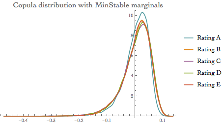
{0.0764216, 0.0882136, 0.0843226, 0.0862706, 0.0832078}

SmoothHistogram[{rsample[[All, 1]], rsample[[All, 2]], 
  rsample[[All, 3]], rsample[[All, 4]], 
  rsample[[All, 5]]}, Automatic, "PDF", 
 PlotLabel -> 
  Style["Copula distribution with MinStable marginals", 16], 
 PlotLegends -> {"Rating A", "Rating B", "Rating C", "Rating D", 
   "Rating E"}]

Extreme value copulae models

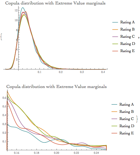
• Extreme value marginals model The probability density for value x in an extreme value distribution is proportional to

  dsoln = Refine[
     Solve[{Mean[ExtremeValueDistribution[a, b]] == \[Eta], 
       Variance[ExtremeValueDistribution[a, b]] == \[Sigma]^2}, {a, b}, 
      Reals], {\[Sigma] > 0}];
  calcmean = 
    Table[dsoln[[2, 1, 
       2]] /. {\[Eta] -> thmean[[i]], \[Sigma] -> tvol[[i]]}, {i, 1, 5}];
  calcvol = 
    Table[dsoln[[1, 2, 
       2]] /. {\[Eta] -> thmean[[i]], \[Sigma] -> tvol[[i]]}, {i, 1, 5}];
  cdExtVal = 
    CopulaDistribution[{"Multinormal", clcovar}, 
     Table[ExtremeValueDistribution[calcmean[[i]], calcvol[[i]]], {i, 1,
        5}]];
  rsample = RandomVariate[cdExtVal, 10^4];
  ircExtValhr = Quantile[rsample, 0.999]
  

{0.223903, 0.250818, 0.228019, 0.255494, 0.249027}

{SmoothHistogram[{rsample[[All, 1]], rsample[[All, 2]], 
   rsample[[All, 3]], rsample[[All, 4]], rsample[[All, 5]]}, 
  Automatic, "PDF", 
  PlotLabel -> 
   Style["Copula distribution with Extreme Value marginals", 16], 
  PlotLegends -> {"Rating A", "Rating B", "Rating C", "Rating D", 
    "Rating E"}, ImageSize -> 350], 
 SmoothHistogram[{rsample[[All, 1]], rsample[[All, 2]], 
   rsample[[All, 3]], rsample[[All, 4]], rsample[[All, 5]]}, 
  Automatic, "PDF", 
  PlotLabel -> 
   Style["Copula distribution with Extreme Value marginals", 16], 
  PlotRange -> {{0.15, 0.25}, All}, 
  PlotLegends -> {"Rating A", "Rating B", "Rating C", "Rating D", 
    "Rating E"}, ImageSize -> 350]}

• StudentT marginals model

The probability density for value x in a Student t distribution with $\nu$ degrees of freedom is proportional to

dsoln = Refine[
   Solve[{Mean[StudentTDistribution[a, b, 10]] == \[Eta], 
     Variance[StudentTDistribution[a, b, 10]] == \[Sigma]^2}, {a, b}, 
    Reals], {\[Sigma] > 0}];
calcmean = 
  Table[dsoln[[1, 1, 
     2]] /. {\[Eta] -> thmean[[i]], \[Sigma] -> tvol[[i]]}, {i, 1, 5}];
calcvol = 
  Table[dsoln[[2, 2, 
     2]] /. {\[Eta] -> thmean[[i]], \[Sigma] -> tvol[[i]]}, {i, 1, 5}];
cdStudent = 
  CopulaDistribution[{"Multinormal", clcovar}, 
   Table[StudentTDistribution[calcmean[[i]], calcvol[[i]], 10], {i, 1,
      5}]];
rsample = RandomVariate[cdStudent, 10^4];
ircStudenthr = Quantile[rsample, 0.999]

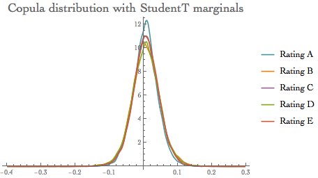
{0.135742, 0.180349, 0.142938, 0.158109, 0.152853}

SmoothHistogram[{rsample[[All, 1]], rsample[[All, 2]], 
  rsample[[All, 3]], rsample[[All, 4]], 
  rsample[[All, 5]]}, Automatic, "PDF", 
 PlotLabel -> 
  Style["Copula distribution with StudentT marginals", 18], 
 PlotLegends -> {"Rating A", "Rating B", "Rating C", "Rating D", 
   "Rating E"}]

Summarising results

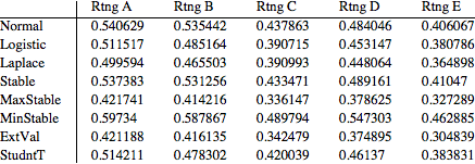
This is the summary of each IRC models discussed above:

ircrates = {ircNormhr, ircLogistichr, ircLaplacehr, ircStablehr, 
   ircMaxStablehr, ircMinStablehr, ircExtValhr, ircStudenthr};
TableForm[ircrates, 
  TableHeadings -> {{"Normal", "Logistic", "Laplace", "Stable", 
     "MaxStable", "MinStable", "ExtVal", "StudntT"}, {"Rtng A", 
     "Rtng B", "Rtng C", "Rtng D", "Rtng E"}}] // TraditionalForm

We observe:

• Variations of the quantile values for each of the specified model

• The values are quite different, especially for the heavy tail distributions (MaxStable, MinStable and Extreme Value)

  • This confirms that the model selection can have a significant impact on the IRC calculation.

IRC Calculation

To obtain the final IRC metric, we need to revalue each cluster portfolio with its quantiled hazard rate. We simulate the cash flow vector per each rating cluster first.

CF = Table[{i, RandomReal[{0.03, 0.08}]}, {i, 0.5, 6, 0.5}];
CFT = Table[
   Table[{i, RandomReal[{0.03, 0.08}]}, {i, 0.5, 6, 0.5}], {5}];
BarChart[CF[[All, 2]], ChartStyle -> "Rainbow", 
 PlotLabel -> Style["Cash flow schedule in cluster A", 20], 
 ChartLabels -> CF[[All, 1]], ImageSize -> 500]

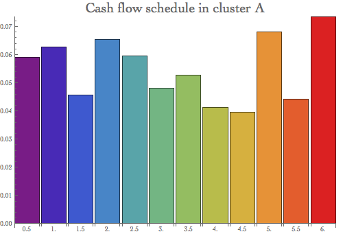
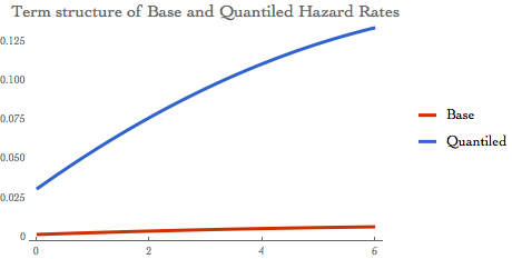
To measure the P&L impact, we evaluate each cluster future cash flows with the "base case" and "quantiled" hazard rates. The difference between these two measures is the portfolio loss due to the credit spread widening, or the incremental risk change.

The IRC is driven by the hazard rate and we can visualise its term structure on the chart below:

il[k_] := {{1, Sqrt[(1/tdur[[k]])]*thmean[[k]]}, {3, 
   Sqrt[(3/tdur[[k]])]*thmean[[k]]}, {tdur[[k]], 
   Sqrt[(tdur[[k]]/tdur[[k]])]*thmean[[k]]}}
ilirc[j_, 
  k_] := {{1, Sqrt[(1/tdur[[k]])]*ircrates[[j, k]]}, {3, 
   Sqrt[(3/tdur[[k]])]*ircrates[[j, k]]}, {tdur[[k]], 
   Sqrt[(tdur[[k]]/tdur[[k]])]*ircrates[[j, k]]}}
InterpBase[k_] := Interpolation[il[k]]
InterpIrc[j_, k_] := Interpolation[ilirc[j, k]]
Plot[{InterpBase[2][x], InterpIrc[4, 2][x]}, {x, 0, 6}, 
  PlotLabel -> 
   Style["Term structure of Base and Quantiled Hazard Rates", 16], 
  PlotTheme -> "Web", PlotLegends -> {"Base", "Quantiled"}] // Quiet

We calculate the IRC as the difference between the CF per cluster risk-adjusted by the "base" case hazard rate and the quantiled one.

The example of the Base Flows:

BaseFlow[n_] := 
 Sum[CFT[[n, i, 2]]*
    Exp[-CFT[[n, i, 1]]*InterpBase[n][CFT[[n, i, 1]]]], {i, 1, 
    Length[CF]}] // Quiet
IrcFlow[j_, n_] := 
 Sum[CFT[[n, i, 2]]*
    Exp[-CFT[[n, i, 1]]*InterpIrc[j, n][CFT[[n, i, 1]]]], {i, 1, 
    Length[CF]}] // Quiet
Table[BaseFlow[i], {i, 1, 5}]

{0.727658, 0.724374, 0.611214, 0.674302, 0.580502}

And these are the similar result for the quantiled hazard rates for each copula model:

TableForm[Table[IrcFlow[i, j], {i, 1, 8}, {j, 1, 5}], 
  TableHeadings -> {{"Normal", "Logistic", "Laplace", "Stable", 
     "MaxStable", "MinStable", "ExtVal", "StudntT"}, {"Rtng A", 
     "Rtng B", "Rtng C", "Rtng D", "Rtng E"}}] // TraditionalForm

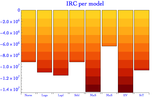
Finally we obtain the total IRC for the entire portfolio as the sum of losses across all clusters. As the graph below shows, the losses are highly dependent on the model choice, with MaxStable and Extreme Value models displaying the highest losses - essentially in multiple of other lighter-tail alternatives.

ModelIrc = 
  Table[Total[
    Table[(IrcFlow[j, i] - BaseFlow[i]), {i, 1, 5}]*10^7], {j, 1, 
    8}];
BarChart[ModelIrc, PlotLabel -> Style["IRC per model", 20], 
 ChartLabels -> {"Norm", "Logs", "Lapl", "Stbl", "MxS", "MnS", "EV", 
   "StT"}, ImageSize -> 500, LabelStyle -> Directive[Blue, 16], 
 PlotRange -> All, 
 ChartElementFunction -> 
  ChartElementDataFunction["SegmentScaleRectangle", "Segments" -> 10, 
   "ColorScheme" -> "SolarColors"]]

Final words.....

• Copulas are practical and tractable methods for construction of multivariate distributions and therefore are ideally suited for the portfolio risk modelling

• We have demonstrated enormous flexibility and power of Wolfram Finance Platform for this task

  • It provides robust and consistent framework for risk modelling in every single aspect

  • It can handle large amount of data, it utilizes optimised protocols and has the speed to obtain the results quickly and efficiently

• The presented approach can be extended in many directions:

  • Volume - adding additional assets / cluster is trivial

  • Definition of the hazard rate process - eg. extension to jump-diffusion / mixtures are easy

  • Use of different liquidity horizons - this is easily achievable through the calibration of the HR stochastic process

  • Copula choices - many alternatives can be offered to test the copula model. StudentT copula, Morgenstern, Frank, Clayton, Gumbel and others are readily available on the Platform. Additional variations can be created through WFP symbolic engine

• Although the modelling approach relies on hazard rate distribution and by-passes rating migration, the latter can be easily included into the framework

  • One can translate the migration matrix into distributional moments or use extensive WFP's linear algebra routines to calculate the cumulative terminal probabilities in time

  • Another suitable option will be modelling of rating transition through Brownian Bridge Process which is specifically designed for this purpose.

Attachments: