Message Boards Message Boards

4
|
9604 Views
|
27 Replies
|
8 Total Likes
View groups...
Share
Share this post:

Different solutions from the same equations in NDSolve ?

Dear community members, I am solving the following set of differential equations with NDSolve. It has been a surprise to me that when solving the problem repeatedly I obtain slightly different solutions. To show this I have repeatedly solve the problem 5 times and plotted the solutions. Any ideas why this may be happening?

DutyCycle[d_, Ts_, t_] := If[0 <= Mod[t, Ts] <= d Ts, 1, 0];
E1 = 16;
Vf = 0.8;
Ts = 100 10^-6;
Td = 0.25;
Rs = 0.001;
Rd = 0.001;
iL0 = 3;
vc0 = 30;
nruns = 5;
nc = 2;
st1 = DutyCycle[Td, Ts, t];
Eqns1 = {iL'[t] == -((Rs (1 - st1) + (Rd st1))/L) iL[t] - 
      st1/L vc[t] + (E1 - (st1 Vf))/L,
                   vc'[t] == st1/C1 iL[t] - 1/(R C1) vc[t], 
    iL[0] == iL0, vc[0] == vc0} /. {R -> 10, L -> 0.2 10^-3, 
    C1 -> 0.2 10^-3};
Do[sol[i] = NDSolve[Eqns1, {iL[t], vc[t]}, {t, 0, nc Ts}], {i, nruns}];
Plot[{Table[vc[t] /. sol[i], {i, nruns}]}, {t, 0, nc Ts}]

Best regards Jesus Rico

27 Replies

The following 'anti-terse' implementation of DutyCycle works for me (i.e. yields a single curve, actually the one reported by Hans Dolaine earlier) on Version 10.0.2.0 and Windows 10.

DutyCycle[d_, Ts_, t_] := 
  Module[{q = t/Ts, n, r}, n = Floor[q]; r = t - n*Ts; 
   If[r < d*Ts, 1., 0.]];

I love the way Module allows to structure complicated expressions. Should speed be a problem, I would go to a compiled version. The original implementation using function Mod should do exactly this. If it fails on some systems there is a bug somewhere, most probably in function Mod.

PS.: I had to discover that now also the original version (using Mod) works fine. So I have no longer any reason to blame function Mod. In my case there was probably a problem with uncleared global definitions that led to the non-uniqueness effect. Hard to see how this should work in detail.

POSTED BY: Ulrich Mutze

Thanks gain for the details to face the problem I have experienced with my commuted circuit. In trying to make my DutyCycle a periodic function I have found a related discussion Periodic piecewise function where periodicity is achieved by the use of the function Mod. One has to be cautious with suggestions given there.

Regards Jesus Rico

Jesus, You're welcome. As I said above, I think it's a bug. I'd suggest you report it. The WRI folks who read Community might not get this far down the page.

Yours, Michael

POSTED BY: Michael Rogers

Thanks. The option Trace Internal is not listed in the documentation, although it does show up when you do Options[Trace].

POSTED BY: Frank Kampas

You can do things like set MaxSteps -> 3 or so to make the output be smaller. It will still be quite large. Of course you don't get the solution all the way to the end and or even to the discontinuity. You could also do separate traces on NDSolve`ProcessEquations and NDSolve`Iterate.

POSTED BY: Michael Rogers

Frank,

I basically used Trace[NDSolve[Eqns1, {iL[t], vc[t]}, {t, 0, nc Ts}], TraceInternal -> True].

This can be helpful, tool: http://mathematica.stackexchange.com/questions/29339/the-clearest-way-to-represent-mathematicas-evaluation-sequence/29340#29340

The basic structure of the computation carried out by NDSolve is described in http://reference.wolfram.com/language/tutorial/NDSolveStateData.html. It helps me know where to look.

POSTED BY: Michael Rogers

How did you figure out what 0 <= Mod[t, 1/10000] <= 0.000025 is translated to?

POSTED BY: Frank Kampas

Part of the issue is that the problem is initialized wrong by NDSolve. Let sol[1] be one solution (the wrong one) and sol[2] be the other (the almost correct one). This is evident in the solutions themselves. The following pairs are the two sides of the equations passed to NDSolve at t == 0; they should be the same, but the derivatives are different. The LHS is wrong for both.

Eqns1 /. Equal -> List /. {iL[t] -> 3, vc[t] -> 30, t -> 0} /. sol[1]
Eqns1 /. Equal -> List /. {iL[t] -> 3, vc[t] -> 30, t -> 0} /. sol[2]
(*
  {{{79985., -74015.}, {-15000., 0.}, {3., 3}, {30., 30}}}
  {{{79985., -74015.}, {-15000., 0.}, {3., 3}, {30., 30}}}
*)

In the second solution, the derivatives are corrected at the first step.

iL'[Take[iL["Grid"] /. First@sol[1], 5]] /. First@sol[1]
iL'[Take[iL["Grid"] /. First@sol[2], 5]] /. First@sol[2]
(*
  {{79985.}, {79985.}, {79985.}, {79981.7}, {79978.5}}
  {{79985.}, {-74015.}, {-74015.}, {-74014.5}, {-74013.6}}
*)

But I cannot say why NDSolve is not deterministic, that is, why it does solves the system two different ways (seemingly at random).

The problem is that the condition 0 <= Mod[t, 1/10000] <= 0.000025 is translated to

Sign@Max[(-1 + NDSolve`CountableCrossingValue[t/Ts])/20000 - 
   t, -0.000025` + (1 - NDSolve`CountableCrossingValue[t/Ts])/20000 + t] < 0

This agrees with 0 <= Mod[t, 1/10000] <= 0.000025 except at t == 0 (and multiples of Ts). So that is the source of the error at the initial value at t == 0. That seems to be a bug.

Using PiecewiseExpand to convert If to Piecewise fixes it. (It has had been mentioned that NDSolve deals with Piecewise more readily than programming constructs like If.) For instance:

Eqns1 = {iL'[t] == PiecewiseExpand[-((Rs (1 - st1) + (Rd st1))/L) iL[t] - 
      st1/L vc[t] + (E1 - (st1 Vf))/L, Assumptions -> 0 <= t <= nc Ts],
   vc'[t] == PiecewiseExpand[st1/C1 iL[t] - 1/(R C1) vc[t], 
     Assumptions -> 0 <= t <= nc Ts],
   iL[0] == iL0, vc[0] == vc0} /. {R -> 10, L -> 0.2 10^-3, 
   C1 -> 0.2 10^-3}

An alternative, more interesting as a check on the analysis above than as a workaround, is to integrated from a small value near zero instead of zero:

NDSolve[Eqns1, {vc, IL}, {t, 1*^-10, nc Ts}]

Either of these approaches produces a consistent result.

POSTED BY: Michael Rogers
DutyCycle[d_, Ts_, t_] := Piecewise[{{1, 0 <= Mod[t, Ts] <= d Ts}}];
E1 = 16;
Vf = 0.8;
Ts = 100 10^-6;
Td = 0.25;
Rs = 0.001;
Rd = 0.001;
iL0 = 3;
vc0 = 30;
nruns = 5;
nc = 2;
st1 = DutyCycle[Td, Ts, t];
Eqns1 = {iL'[t] == -((Rs (1 - st1) + (Rd st1))/L) iL[t] - 
      st1/L vc[t] + (E1 - (st1 Vf))/L, 
    vc'[t] == st1/C1 iL[t] - 1/(R C1) vc[t], iL[0] == iL0, 
    vc[0] == vc0} /. {R -> 10, L -> 0.2 10^-3, C1 -> 0.2 10^-3};
Do[sol[i] = NDSolve[Eqns1, {iL[t], vc[t]}, {t, 0, nc Ts}], {i, nruns}];
(*Plot[{Table[vc[t]/.sol[i],{i,nruns}]},{t,0,nc Ts}]*)
Table[Plot[vc[t] /. sol[i], {t, 0, nc Ts}], {i, nruns}]

enter image description here

POSTED BY: Frank Kampas

Hi Frank,

you are quite right. $Mod$ also seems to cause problems. As you say:

DutyCycle[d_, Ts_, t_] := Piecewise[{{1, 0 <= Mod[t, Ts] <= d Ts}}];

does not seem to work. And

DutyCycle[d_, Ts_, t_] := Ceiling[-(Mod[t, Ts] - Ts d)]

does not work either. So there is a problem with $Mod$. But

DutyCycle[d_, Ts_, t_] := HeavisideTheta[Sin[2 Pi/Ts*t + Pi*d] - Sin[Pi*d]];

and

DutyCycle[d_, Ts_, t_] := If[Sin[2 Pi/Ts*t + Pi*d] - Sin[Pi*d] > 0, 1, 0];

do work; in spite of the latter having the "If". Curiously enough,

DutyCycle[d_, Ts_, t_] := HeavisideTheta[SawtoothWave[t/Ts - d] - (1 - d)];

does not work. In the following case, however, there is no $Mod$ and things still go wrong:

DutyCycle[d_, Ts_, t_] := If[IntervalMemberQ[IntervalUnion @@ Table[Interval[{k Ts, Ts d + k Ts}], {k, 0, 4}], t], 1, 0]; 

This last one, I couldn't even make work with Piecewise, i.e.

DutyCycle[d_, Ts_, t_] := Piecewise[{{1, IntervalMemberQ[IntervalUnion @@ Table[Interval[{k Ts, Ts d + k Ts}], {k, 0, 4}], t]}}];

does not work either.

DutyCycle[d_, Ts_, t_] := Evaluate[Piecewise[Flatten[Table[{{1, (k - 1) Ts < t < (k + Td) Ts}, {0, (k + Td) Ts < t < (k + 1) Ts}}, {k, -2,3} ], 1]]];

does work, but

DutyCycle[d_, Ts_, t_] := Piecewise[Flatten[Table[{{If[Evaluate[0 < Mod[t, Ts] < d Ts], 1, 0], (k - 1) Ts < t < (k + d) Ts}, { If[Evaluate[0 < Mod[t, Ts] < d Ts], 1, 0], (k + d) Ts < t < (k + 1) Ts}}, {k, -2, 3} ], 1]];

does not - making the case against $Mod$ even stronger.

If I have not made a mistake, all of these functions should be identical in the interval of interest, say from $0$ to $nc Ts$, which you can test by running

Plot[{DutyCycle[Td, Ts, t]}, {t, -nc Ts, 2 nc Ts}]

--- some work some don't.

Cheers,

Marco

PS: I had some other examples of writing this function, but unfortunately, the session died on me when I wanted to post.

POSTED BY: Marco Thiel

Interestingly, the two different results from the original formulation alternate.
enter image description here

POSTED BY: Frank Kampas

...but not on my system :-)

POSTED BY: Hans Dolhaine

Hi Frank,

I don't think that in general the solutions alternate.

enter image description here

Also, the same behaviour occurs on MMA 9. But all of this can be "fixed", by using the Piecewise function which is recommended for ODEs. If should be avoided in these cases.

Best wishes,

Marco

POSTED BY: Marco Thiel

When you went to the Piecewise function, you also got rid of the Mod function inside. Recently I was using CompilePrint to look at a compiled Piecewise function and an equivalent If statement and they looked the same. Could the Mod be the problem?

POSTED BY: Frank Kampas

The code I have that uses FindMinimum and doesn't give reproducible results for large problems involves a function with a discontinuous first derivative from a Max function. Perhaps discontinuity is the cause of the problem.

POSTED BY: Frank Kampas

Marco, Excellent demonstration, big thanks!. I will use the suggested definition as the basis for my periodic DutyCycle function. Also, the solution you have obtained coincides with my semi analytical one.

Best regards Jesus Rico

Hi,

I suspect that this is a numerical issue related to the If function. If you plot the DutyCycle function with your parameters over time you get:

Plot[DutyCycle[Td, Ts, t], {t, -nc Ts, nc Ts}]
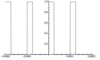
enter image description here

As 
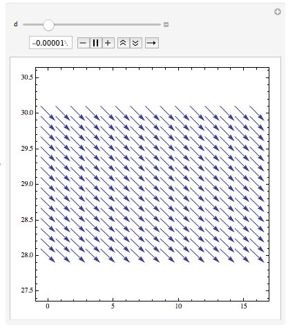
$t$ changes from negative to positive the vector field changes.

Manipulate[VectorPlot[Evaluate[{-((Rs (1 - st1) + (Rd st1))/L) iL - st1/L vc + (E1 - (st1 Vf))/L /. {R -> 10, L -> 0.2 10^-3, C1 -> 0.2 10^-3, t -> d}, st1/C1 iL - 1/(R C1) vc} /. {R -> 10, L -> 0.2 10^-3, C1 -> 0.2 10^-3, t -> d}], {iL, 0, 16}, {vc, 28, 30}], {d, -0.1 nc Ts, 0.1 nc Ts}]

enter image description here

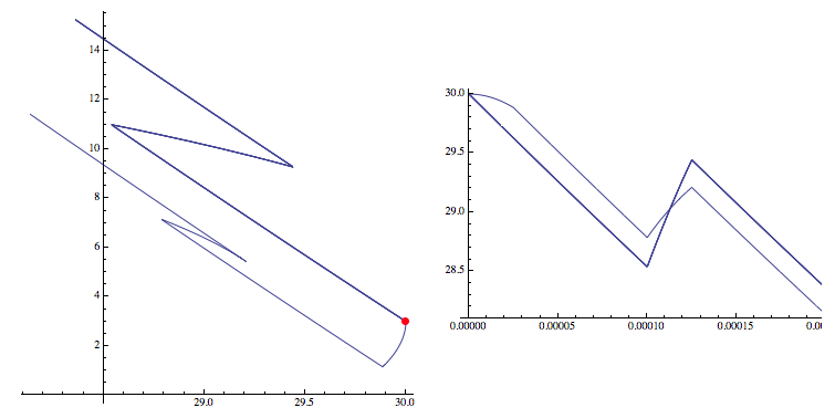
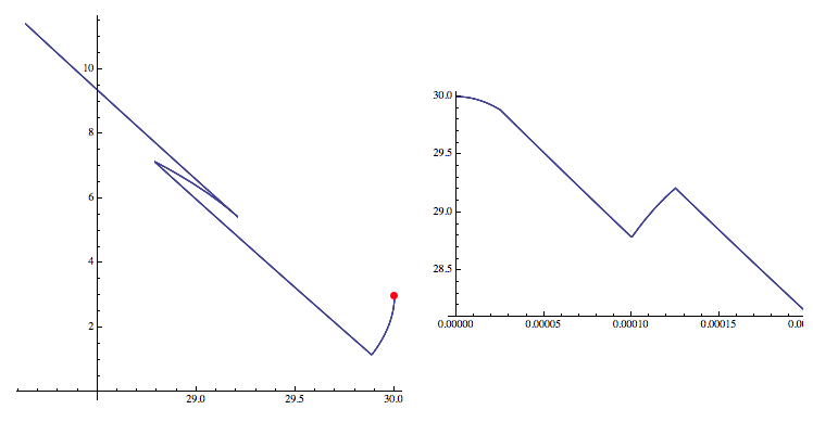
If you plot the trajectory in the phase plane (the initial point is marked by a red dot)

DutyCycle[d_, Ts_, t_] := If[0 <= Mod[t, Ts] <= d Ts, 1, 0];
E1 = 16;
Vf = 0.8;
Ts = 100 10^-6;
Td = 0.25;
Rs = 0.001;
Rd = 0.001;
iL0 = 3;
vc0 = 30;
nruns = 5;
nc = 2;
st1 = DutyCycle[Td, Ts, t];
Eqns1 = {iL'[t] == -((Rs (1 - st1) + (Rd st1))/L) iL[t] - 
      st1/L vc[t] + (E1 - (st1 Vf))/L, 
    vc'[t] == st1/C1 iL[t] - 1/(R C1) vc[t], iL[0] == iL0, 
    vc[0] == vc0} /. {R -> 10, L -> 0.2 10^-3, C1 -> 0.2 10^-3};
Do[sol[i] = NDSolve[Eqns1, {iL[t], vc[t]}, {t, 0, nc Ts}], {i, nruns}];
GraphicsRow[{ParametricPlot[{Table[{vc[t], iL[t]} /. sol[i], {i, 
      nruns}]}, {t, 0, nc Ts}, AspectRatio -> 1, ImageSize -> Medium, 
   Epilog -> {Red, PointSize[Large], Point[{vc0, iL0}]}], 
  Plot[{Table[vc[t] /. sol[i], {i, nruns}]}, {t, 0, nc Ts}, 
   PlotPoints -> 40, ImageSize -> Medium]}]

you get

enter image description here

If you start anywhere near (but numerically close to) time zero, you only obtain one solution. So

DutyCycle[d_, Ts_, t_] := If[0 <= Mod[t, Ts] <= d Ts, 1, 0];
E1 = 16;
Vf = 0.8;
Ts = 100 10^-6;
Td = 0.25;
Rs = 0.001;
Rd = 0.001;
iL0 = 3;
vc0 = 30;
nruns = 5;
nc = 2;
st1 = DutyCycle[Td, Ts, t];
Eqns1 = {iL'[t] == -((Rs (1 - st1) + (Rd st1))/L) iL[t] - 
      st1/L vc[t] + (E1 - (st1 Vf))/L, 
    vc'[t] == st1/C1 iL[t] - 1/(R C1) vc[t], iL[10^-10] == iL0, 
    vc[10^-10] == vc0} /. {R -> 10, L -> 0.2 10^-3, C1 -> 0.2 10^-3};
Do[sol[i] = NDSolve[Eqns1, {iL[t], vc[t]}, {t, 10^-10, nc Ts}], {i, 
   nruns}];
GraphicsRow[{ParametricPlot[{Table[{vc[t], iL[t]} /. sol[i], {i, 
      nruns}]}, {t, 0, nc Ts}, AspectRatio -> 1], 
  Plot[{Table[vc[t] /. sol[i], {i, nruns}]}, {t, 0, nc Ts}, 
   PlotPoints -> 40]}]

and

DutyCycle[d_, Ts_, t_] := If[0 <= Mod[t, Ts] <= d Ts, 1, 0];
E1 = 16;
Vf = 0.8;
Ts = 100 10^-6;
Td = 0.25;
Rs = 0.001;
Rd = 0.001;
iL0 = 3;
vc0 = 30;
nruns = 5;
nc = 2;
st1 = DutyCycle[Td, Ts, t];
Eqns1 = {iL'[t] == -((Rs (1 - st1) + (Rd st1))/L) iL[t] - 
      st1/L vc[t] + (E1 - (st1 Vf))/L, 
    vc'[t] == st1/C1 iL[t] - 1/(R C1) vc[t], iL[-10^-10] == iL0, 
    vc[-10^-10] == vc0} /. {R -> 10, L -> 0.2 10^-3, 
    C1 -> 0.2 10^-3};
Do[sol[i] = NDSolve[Eqns1, {iL[t], vc[t]}, {t, -10^-10, nc Ts}], {i, 
   nruns}];
GraphicsRow[{ParametricPlot[{Table[{vc[t], iL[t]} /. sol[i], {i, 
      nruns}]}, {t, 0, nc Ts}, AspectRatio -> 1], 
  Plot[{Table[vc[t] /. sol[i], {i, nruns}]}, {t, 0, nc Ts}, 
   PlotPoints -> 40]}]

both give

enter image description here

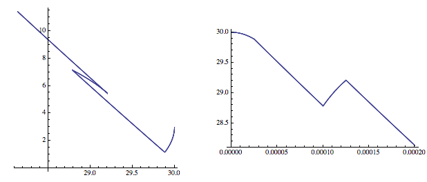
Ok, now we can try to define the DutyCycle function using Piecewise, which is recommended in the context of ODES.

DutyCycle[d_, Ts_, t_] := 
  Piecewise[{{1, t < d Ts}, {0, t < d Ts}, {1, 5/4 Ts > t > Ts}, {0, 
     t > 5/4 Ts}}];
E1 = 16;
Vf = 0.8;
Ts = 100 10^-6;
Td = 0.25;
Rs = 0.001;
Rd = 0.001;
iL0 = 3;
vc0 = 30;
nruns = 5;
nc = 2;
st1 = DutyCycle[Td, Ts, t];
Eqns1 = {iL'[t] == -((Rs (1 - st1) + (Rd st1))/L) iL[t] - 
      st1/L vc[t] + (E1 - (st1 Vf))/L, 
    vc'[t] == st1/C1 iL[t] - 1/(R C1) vc[t], iL[0] == iL0, 
    vc[0] == vc0} /. {R -> 10, L -> 0.2 10^-3, C1 -> 0.2 10^-3};
Do[sol[i] = NDSolve[Eqns1, {iL[t], vc[t]}, {t, 0, nc Ts}], {i, nruns}];
GraphicsRow[{ParametricPlot[{Table[{vc[t], iL[t]} /. sol[i], {i, 
      nruns}]}, {t, 0, nc Ts}, AspectRatio -> 1, ImageSize -> Medium, 
   Epilog -> {Red, PointSize[Large], Point[{vc0, iL0}]}], 
  Plot[{Table[vc[t] /. sol[i], {i, nruns}]}, {t, 0, nc Ts}, 
   PlotPoints -> 40, ImageSize -> Medium]}]

This results in

enter image description here

So not there is only one solution, which I hope coincides with your favourite solution.

Cheers,

Marco

POSTED BY: Marco Thiel

Frank I am running this on a Mac Pro, My operating system is Yosemite but I do not know how to get the version (sorry I am not good at that) I have mathematica 10.0 but I have obtained the same inconsistency in Wolfram Desktop 10.0.1. Jesus

I get two solutions on my MacBookAir, running Mathematica 10.2 under OS X Yosemite Version 10.10.5

POSTED BY: Frank Kampas

Jesus, What operating system and what version of Mathematica are you using? That info may help understand the problem since Hans doesn't see it. Hans, same question to you.

POSTED BY: Frank Kampas

Hello Frank,

I use Windows 7 and Mathematica 7.0.0. .

Running it 15 times yieds always the same plot:

DutyCycle[d_, Ts_, t_] := 
 If[0 <= Mod[t, Ts] <= d Ts, 1, 0]; E1 = 16; Vf = 0.8; Ts = 
 100 10^-6; Td = 0.25; Rs = 0.001; Rd = 0.001; iL0 = 3; vc0 = 30; \
nruns = 15; nc = 2; st1 = 
 DutyCycle[Td, Ts, 
  t]; Eqns1 = {iL'[t] == -((Rs (1 - st1) + (Rd st1))/L) iL[t] - 
     st1/L vc[t] + (E1 - (st1 Vf))/L, 
   vc'[t] == st1/C1 iL[t] - 1/(R C1) vc[t], iL[0] == iL0, 
   vc[0] == vc0} /. {R -> 10, L -> 0.2 10^-3, C1 -> 0.2 10^-3}; Do[
 sol[i] = NDSolve[Eqns1, {iL[t], vc[t]}, {t, 0, nc Ts}], {i, 
  nruns}]; Plot[{Table[vc[t] /. sol[i], {i, nruns}]}, {t, 0, nc Ts}]

enter image description here

POSTED BY: Hans Dolhaine

Frank I now which of the two is the most accurate because I have worked out some semi analytical solutions and I really can continue with what I am doing but it has being a little intreging why a sophisticated algorithm such as NDSolve behaves a little randomly. I guess that this little problem may be indeed very important when solving the same system near chaotic operating points. Thanks

Jesus Rico

What happens if you substitute the two solutions into the differential equations? You could calculate and plot an error term for each equation to see if either of the solutions is correct.

POSTED BY: Frank Kampas

Hi again! My equations may be chaotic but not for the parameters I am using in this case. And Yes, I got two different plots with mathematica 10.2 but in which run the solution will change is a random event. If they were only two different solutions, why is that??

Best Regards

Jesus Rico

I see two different plots when I run the code using Mathematica 10.2 running on Windows 8.1 - 64.

POSTED BY: Frank Kampas

I did 8 plots, and they were all the same (Mathematica Version 7) Regards H. Dolhaine

POSTED BY: Hans Dolhaine

Are your equations chaotic? I get different solutions from FindMinimum for complex problems if I run them repeatedly.

POSTED BY: Frank Kampas
Reply to this discussion
Community posts can be styled and formatted using the Markdown syntax.
Reply Preview
Attachments
Remove
or Discard

Group Abstract Group Abstract