As a Mathematics student at the Universitat Autònoma de Barcelona, I have had the opportunity to take up an Erasmus Internship at the Mathematics Department of the University of Aberdeen, supervised by Dr Marco Thiel, from June to September of 2015, in which I have covered approximately 260 hours of work.

The purpose of this Internship was to get acquainted with the Mathematica computer programme and to be able to make real-life applications of its features. My supervisor first introduced me to a glioma-simulating project, which is a type of cancer that affects the brain. On diagnosis, such condition has a devastating life expectancy of 1 to 3 years. So from the beginning, being part of this project seemed very attractive to me and I believed that detailed research on it could potentially be highly useful for Physical Sciences, Medicine and surely to those patients suffering from the disease.

First of all, I learned about the Mathematica computer programme, the glioma tumour itself and its possible mathematical models as well as understanding the behaviour of the diffusion equations, given that the glioma may be described by one of them. Secondly, I familiarised myself with image-processing as cleaning pictures would play a major role in my work. And finally, once I managed these initial steps, I was able to begin working on the modelling of a glioma tumour in 2D and 3D afterwards. This is my small contribution that I hope you will find useful.

Introduction to a glioma

A glioma is a neoplasia of glial cells, normally located in the superior cerebral hemisphere, even though it can be found anywhere throughout the brain and occasionally in the spinal cord, since it rarely spreads outside of the brain. This abnormal growth of the tissue generally forms a tumour, which could be classified as a low-grade glioma (benign tumour) or as a high-grade glioma (malignant tumour).

In this research work, we focus on analysing the behaviour of malignant tumours only and we also establish that the glioma does not spread outside of the brain. We will use the mathematical model described in the book “Mathematical Biology (Vol II: Spatial Models and Biomedical Applications)”, written by J. D. Murray:

$\frac{dc\left(t,\bar{x}\right)}{dt}=\nabla\left(D(\bar{x}) \nabla c\left(t,\bar{x}\right) \right)+ \rho c\left(t,\bar{x}\right)$,

where $c(t,\bar{x})$ is the number of cells at position $\bar{x}$ and time $t$, $D(\bar{x})$ ( $\frac{distance^2}{time}$) is the diffusion coefficient of cells depending on the position and considering that the spread rate is approximately five times greater in the white matter regions than in the grey matter ones, and $\rho$ ( $time^{-1}$) is the growth rate of cancer cells given its proliferation and death. Regarding the initial condition of the project, we will use a Gaussian distribution and in regards of the boundary condition, it is indicated in the book mentioned above that:

${\bf n} \cdot D(\bar{x}) \nabla c\left(t,\bar{x}\right) = 0 \qquad \text{for}\; \bar{x}\; \text{on}\; \partial B$,

where $\partial B$ is the brain boundary, ${\bf n}$ is the normal vector at $\partial B$, and $D(\bar{x})$ and $c\left(t,\bar{x}\right)$ as previously stated. However, we will not make use of this boundary condition, instead we will simplify it as explained below.

Two Dimension Imaging (2D)

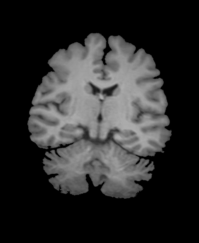
In order to become familiar with the Mathematica programme, its equations and parameters, we will start analysing the behaviour of a glioma in 2D. A valuable introduction on this topic has already been made by Dr Marco Thiel in his paper ”Simulating Brain Tumor Growth with Mathematica 10”, where he explains in detail every necessary step (including simplified boundary condition) to achieve glioma imaging in 2D.

Nonetheless, on this project I have added some subtle changes as follows:

1.Enhance image cleaning:

img1 = Import["~/Desktop/brain.jpg"];
img2 = Sharpen[ColorConvert[img1, "Grayscale"]];
img = ImageMultiply[img2, SelectComponents[FillingTransform@Binarize[img2], "Area", -1]]

2.Increase the image contrast to obtain an exponential, non-linear diffusion coefficient:

ic = ImageAdjust[img, {1, 0.5}];
coeff = ListInterpolation[ImageData[ic]];

and $coeff^{10}$ will be used to male the diffusion coefficient clearer.

3.Check the diffusion equation orientation depending on the image:

ContourPlot[coeff[x, y], {x, 1., 798.}, {y, 1., 654}]

The orientation shown is not correct, and to amend it it should just be applied:

ContourPlot[coeff[799. - x, y], {y, 1., 654}, {x, 1., 798.}]

4.Adjustment of the parameters to the new dimensions.

The "Mathematical Biology (Vol II: Spatial Models and Biomedical Applications)” book provides the diffusion coefficient values in both white matter and grey matter regions and the growth cell rate, which is the value of both parameters according to the grade of the glioma.

The cells growth rate is $day^{-1}$, which indicates that we will see how the glioma grows in day intervals. Regarding the diffusion coefficient, its unit is $\frac{cm^2}{day}$. Additionally, we will be working within a $1x1$ size square, which neither approximates to real dimensions nor to real proportions. Therefore, we should reformulate the diffusion coefficient if we are to find our image’s dimensions in reality. In this case, I have searched the number of pixels that fits to the brain width in the image and have related this number to the brain’s real width, which is approximately 14cm. Once the pixels-cm rate has been found, it is possible to obtain the full-size image. Finally we divide the diffusion coefficient by the product of the dimensions of the real image. For example, if we want to study a glioma with a diffusion coefficient of $0.005\frac{cm^2}{day}$, we will use $\frac{0.005}{33.9x41.3} \frac{u^2}{day}$, ( $u=unit$).

So to conclude this section, we are now able to solve the PDE for two dimensions by applying all the above changes to "Simulating Brain Tumor Growth with Mathematica 10".

boundaries = {-y, y - 1, -x, x - 1};

\[CapitalOmega] =ImplicitRegion[And @@ (# <= 0 & /@ boundaries), {x, y}];

sols = NDSolveValue[{{Div[(0.005/33.9/41.3)*(coeff[797.*x + 1., 653.*y + 1.])^10*Grad[u[t, x, y], {x, y}], {x, y}] - D[u[t, x, y], t] + 0.012*u[t, x, y] == NeumannValue[0., x >= 1. || x <= 0. || y <= 0. || y >= 1.]}, {u[0, x, y] == Exp[-1000. ((x - 0.6)^2 + (y - 0.6)^2)]}}, u, {x, y} \[Element] \[CapitalOmega], {t, 0, 200}, Method -> {"FiniteElement", "MeshOptions" -> {"BoundaryMeshGenerator" -> "Continuation",MaxCellMeasure -> 0.002}}];

frames = Table[ImageCompose[img, {ContourPlot[sols[i, 1 - x, y], {y, 0, 1}, {x, 0, 1}, PlotRange -> {{0, 1}, {0, 1}, {0.01, All}}, PlotPoints -> 1, Contours -> 20, ContourLines -> False, AspectRatio -> 798./654., ColorFunction -> "Temperature", Frame -> False], 0.6}], {i, 0, 200, 20}];

ListAnimate[frames]

Three Dimension Imaging (3D)

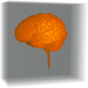
Once we understand the behaviour of a 2D glioma, we can add on another dimension to achieve a more accurate approximation to reality. In order to carry out the simulation of a 3D glioma growth, brain-scanner images are required to obtain a 3D brain and, as I did in 2D imaging, the diffusion equation will be needed too. We begin cleaning up the scanned images. After only the brain is shown in the pictures, we can then represent a 3D brain:

obj = Import["~/Desktop/brain2.tiff"];

brainM = Image3D[obj]

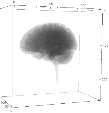
And the glioma will be shown in the 3D image by:

Export["brainM.tiff", brainM];

b = Graphics3D[{Opacity[0.01],Raster3D[ImageData@ColorNegate@Binarize@Import["C:/Users/Laura/Documents/brainM.tiff", "Image3D"]]}, Axes -> True]

Same as I did with the 2D imaging, we will increase the brain contrast colour to get a sharper diffusion coefficient:

ib = ImageAdjust[brainM, {1, 0.5}];

Then the diffusion coefficient is reached:

coeff = ListInterpolation[ImageData[ib]];

We check the coefficient orientation according to the brain, this will enable to show how the tumour spreads:

bb = ContourPlot3D[
   coeff[x, y, z], {x, 1., 135.}, {y, 1., 256.}, {z, 1., 256.}, 
   BoxRatios -> {135., 256., 256.}];

Show[b, bb]

Some changes are required to fit them all:

bb = ContourPlot3D[
   coeff[x, y, z], {z, 1., 256.}, {y, 1., 256.}, {x, 1., 135.}, 
   BoxRatios -> {256., 256., 135.}];

Show[b, bb]

Once all these steps have been completed, we can proceed to solve our differential equation, taking into account the boundary conditions $NeumannValue[0.,x>=1.||x<=0.||y<=0.||y>=1.||z<=0.||z>=1.]$, the initial condition (Gauss distribution), and the parameters, which are to be reformulated again:

$\frac{parameters(cm^2/days)}{24.15x12.73}=newParameter(u^2/days)$.

Regarding the parameters, we will use the ones specified in the “Mathematical Biology (Vol II: Spatial Models and Biomedical Applications)” book;

High-grade glioma: $\rho=1.2x10^{-2} days^{-1}$ i $dcw=1.3x10^{-3} \frac{cm^2}{days}$ ( $dcw$=diffusion coefficient in white matter)

Slow-grade glioma: $\rho=1.2x10^{-3} days^{-1}$ i $dcw=1.3x10^{-4} \frac{cm^2}{days}$ ( $dcw$=diffusion coefficient in white matter)

solsHH = NDSolveValue[{{Div[(0.0013/24.15/
          12.73)*(coeff[134.*x + 1., 255.*y + 1, 255.*z + 1.])^10*
        Grad[u[t, x, y, z], {x, y, z}], {x, y, z}] - 
      D[u[t, x, y, z], t] + 0.012*u[t, x, y, z] == 
     NeumannValue[0., 
      x >= 1. || x <= 0. || y <= 0. || y >= 1. || z <= 0. || 
       z >= 1.]}, {u[0, x, y, z] == 
     50 Exp[-400. ((x - 0.4)^2 + (y - 0.4)^2 + (z - 0.4)^2)]}}, 
  u, {x, y, z} \[Element] Cuboid[{0, 0, 0}, {1, 1, 1}], {t, 0, 200}, 
  Method -> {"FiniteElement", 
    "MeshOptions" -> {"BoundaryMeshGenerator" -> "Continuation", 
      MaxCellMeasure -> 0.002}}]

framesHH = 
  Table[Show[b, 
    ContourPlot3D[
     solsHH[i, x/134., y/255., z/255.] == 9.5, {z, 0., 255.}, {y, 0., 
      255.}, {x, 0., 134.}, 
     PlotRange -> {{0., 255.}, {0., 255.}, {0., 134.}, {0.01, All}}, 
     PlotPoints -> 5, Contours -> 1, ColorFunction -> "Temperature", 
     BoxRatios -> {255., 255., 134.}]], {i, 0, 200, 20}];

solsLL = NDSolveValue[{{Div[(0.00013/24.15/
          12.73)*(coeff[134.*x + 1., 255.*y + 1., 255.*z + 1.])^10*
        Grad[u[t, x, y, z], {x, y, z}], {x, y, z}] - 
      D[u[t, x, y, z], t] + 0.0012*u[t, x, y, z] == 
     NeumannValue[0., 
      x >= 1. || x <= 0. || y <= 0. || y >= 1. || z <= 0. || 
       z >= 1.]}, {u[0, x, y, z] == 
     50 Exp[-400. ((x - 0.4)^2 + (y - 0.4)^2 + (z - 0.4)^2)]}}, 
  u, {x, y, z} \[Element] Cuboid[{0, 0, 0}, {1, 1, 1}], {t, 0, 200}, 
  Method -> {"FiniteElement", 
    "MeshOptions" -> {"BoundaryMeshGenerator" -> "Continuation", 
      MaxCellMeasure -> 0.002}}]

framesLL = 
  Table[Show[b, 
    ContourPlot3D[
     solsLL[i, x/134., y/255., z/255.] == 9.5, {z, 0., 255.}, {y, 0., 
      255.}, {x, 0., 134.}, 
     PlotRange -> {{0., 255.}, {0., 255.}, {0., 134.}, {0.01, All}}, 
     PlotPoints -> 5, Contours -> 1, ColorFunction -> "Temperature", 
     BoxRatios -> {255., 255., 134.}]], {i, 0, 200, 20}];

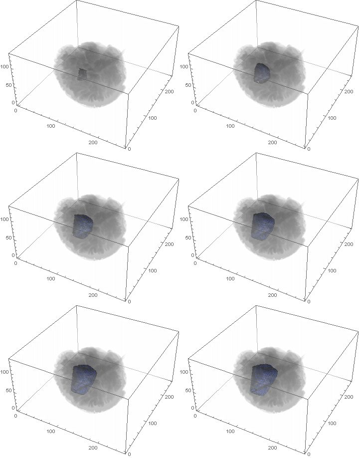
VideoHH = ListAnimate[framesHH]

VideoLL = ListAnimate[framesLL]

Conclusion

We can clearly see the difference between the two gliomas growth velocities displayed on the above videos over a period of just 200 days. Following steps on this topic might help to calculate the volume of the tumour and therefore to elaborate a time-volume graphic. Thus, the patient’s life expectancy on diagnosis could be predicted, given that death normally occurs when the volume of the glioma is higher than a sphere, radius 3cm. Moreover, the boundary condition specified in the book could be altered to observe how it affects the outcome. Finally, we could study the behaviour of the glioma by using the non-linear differential equation $\frac{dc\left(t,\bar{x}\right)}{dt}=\nabla\left(D(\bar{x}) \nabla c\left(t,\bar{x}\right) \right)+ \rho c\left(t,\bar{x}\right)\left(1-\frac{c\left(t,\bar{x}\right)}{K}\right)$,where K is the limiting number of cells that the tissue can hold, and see whether any significant impact has been made.

Cheers,

Laura Carrera Escalé

carrera.escale@gmail.com