At Wolfram Science Summer School 2013 that is currently in progress, we came by an interesting system mentioned in the
NKS book on the page 1059. It is a quantum block cellular automaton (CA) with unitary evolution that preserves magnitude of complex field. I thought it would be interesting to implement it. It is rather rare we come by a clear simple design for a quantum CA. Below initial conditions are to complex numbers IC1 and IC2 placed on background of zeros. The rule number runs continuous space from 0 to 2Pi and is the angle of unitary operator.
Manipulate[
data = NestList[step[a], ArrayPad[{IC1[[1]] + I IC1[[2]], 0, 0, 0, 0, 0, 0, 0, 0, 0, 0, IC2[[1]] + I IC2[[2]]}, {15, 15}], 30];
Grid[{{
ArrayPlot[Abs[data], ColorFunction -> "DarkRainbow", Mesh -> True, Frame -> False, PlotRangePadding -> 0, ImageSize -> 300], ArrayPlot[Arg[data], ColorFunction -> "DarkRainbow", Mesh -> True, Frame -> False, PlotRangePadding -> 0, ImageSize -> 300]
}}, Spacings -> 0] ,
{{a, 2.94, "rule"}, 0, 2 Pi, ImageSize -> Tiny} ,
{IC1, {-1, -1}, {1, 1}} ,
{IC2, {-1, -1}, {1, 1}} ,
FrameMargins -> 0 , ControlPlacement -> Left ,
SaveDefinitions -> True , Initialization -> (
evo[x_][y_] := {{Cos[x], I Sin[x]}, {I Sin[x], Cos[x]}}.y;
stepA[a_][l_] := Flatten[evo[a] /@ Partition[l, 2, 2, 1]];
stepB[a_][l_] := RotateRight[Flatten[evo[a] /@ Partition[RotateLeft[l], 2, 2, 1]]];
step[a_][l_] := stepB[a][stepA[a][l]] )]
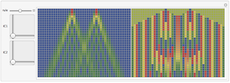
The two plots are amplitude and phase of the evolution. Now lets verify that evolution is indeed unitary. Variable data (the evolution steps) is global so we could just simply apply:
Tr[Abs[#]^2] & /@ data
(* Out[] = {0.0325, 0.0325, 0.0325, ..... } *)


