Iterative procedures are many times very sensitive to starting values. Sometimes one has to be very close to the correct estimates and sometime one just needs to start with the right sign. My guess that NonlinearModelFit uses 1 as the starting value for all parameters. If one uses -1 for the starting value for d, a good fit results.

Z = NonlinearModelFit[data, Ic, {x, { d, -1}, j}, T];
Z["BestFitParameters"]
Z["BestFit"]
Show[Plot[Z[T], {T, 4, 300}, PlotRange -> All], ListPlot[data] ]

Hi SG,

I am not sure, whether this is right, but it could be that your function does not really fit the points very well. There is a pole at 0, which means that the functions quickly increases to infinity and if the points for larger T are fitted correctly, you get the first two very (!) wrong. So the algorithm decides to find a compromise.

If you ignore the first two points the fits look very different:

data = {{4, 31.44748412}, {10, 25.77945826}, {20, 15.72330464}, {30, 
    11.01076634}, {40, 8.079719552}, {80, 4.313645621}, {120, 
    2.704975269}, {180, 1.954029677}, {240, 1.094268257}, {300, 1}};
Ic = (0.011461162748288768 d^2 x)/((1 + E^(-0.9149849674149166/T) + 
     E^((7.241129616220129*^22 (-6.3179712*^-24 - d/
        1000000000000000000000000))/T) + E^((
     7.241129616220129*^22 (-6.3179712*^-24 - d/
        3000000000000000000000000 - j/500000000000000000000000))/
     T)) T);
Z = NonlinearModelFit[data, (
  0.011461162748288768 d^2 x)/((1 + E^(-0.9149849674149166/T) + E^((
     7.241129616220129*^22 (-6.3179712*^-24 - d/
        1000000000000000000000000))/T) + E^((
     7.241129616220129*^22 (-6.3179712*^-24 - d/
        3000000000000000000000000 - j/500000000000000000000000))/
     T)) T), {x, d, j}, T, 
  Weights -> {0.0, 0.0, 1, 1, 1, 1, 1, 1, 1, 1}, MaxIterations -> 1000]
Show[ListPlot[data], 
 Plot[Z[T], {T, 0, 300}, PlotRange -> {All, {0, 35}}]]
Show[ListPlot[data], 
 Plot[2.5*Z[T], {T, 0, 300}, PlotRange -> {All, {0, 35}}]]

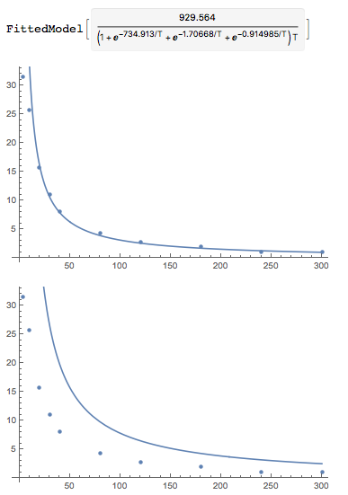
Now, if you multiply by 2.5 it becomes obvious that the fit is not good anymore.

So I think that this effect might come from the fact that the pole at zero causes large deviations from the measurements, or in other words that your function, with the degrees of freedom that you chose, is not a good model for the measurement.

Cheers,

Marco