The world was not as easy as I expected. Here are the steps I took to map it into the flattened icosahedron so I can print it out, cut it out, fold it and tape it to my shirt for Halloween.
Start out with the world in lat-long.
world2d = CountryData["World", "Polygon"];
Convert to 3d.
world3d = N[world2d[[1, 1]]] /. {x_Real, y_Real} :> ({Cos[#2] Cos[#], Sin[#2] Cos[#], Sin[#]} &[x*Degree, y*Degree]);
Some modified data from PolyhedronData giving the two and three dimensional coordinates of the vertices and face indices.
v3 = PolyhedronData["Icosahedron", "VertexCoordinates"];
i3 = PolyhedronData["Icosahedron", "FaceIndices"];
f3 = v3[[#]] & /@ i3;
v2 = PolyhedronData["Icosahedron", "NetCoordinates"];
i2b = {{1, 6, 7}, {13, 6, 12}, {2, 7, 8}, {14, 7, 13}, {3, 8, 9}, {15, 8, 14}, {4, 9, 10}, {16, 9, 15}, {5, 10, 11}, {17, 10, 16}, {6, 13, 7}, {13, 12, 18}, {7, 14, 8}, {14, 13, 19}, {8, 15, 9}, {15, 14, 20}, {9, 16, 10}, {16, 15, 21}, {10, 17, 11}, {17, 16, 22}}
f2b = v2[[#]] & /@ i2b;
f3tof2b = {1, 3, 5, 7, 9, 18, 20, 12, 14, 16, 11, 13, 15, 17, 19, 8, 10, 2, 4, 6};
Convert 3d coordinates to the face index and local face 2d coordinates.
FacePlanes =  Apply[Function[{a, b, c}, {Cross[a, b], Cross[b, c], Cross[c, a]}],  N@f3, {1}];
FaceMeans = Apply[Function[{a, b, c}, Mean[{a, b, c}]], N@f3, {1}];
FaceInverses = Apply[Function[{a, b, c}, Inverse[{Mean[{a, b, c}], b - a, c - a}][[All, 2 ;; 3]]], N@f3, {1}];
FaceCoord[p_] := With[{coords = Select[Table[{i, FacePlanes[[i]].p}, {i, 20}], Min[#[[2]]] >= 0 &,1][[1]]},
{coords[[1]],  p.FaceInverses[[coords[[1]]]] (.571175/(p.FaceMeans[[coords[[1]]]]))}]

worldpattern0 = world3d /. {x_Real, y_Real, z_Real} :> FaceCoord[{x, y, z}];
Convert the index plus coordinates to the plane. Also split the lists of coordinates so that lines don't cross faces weirdly.
ProjCoord[{ind_, {x_, y_}}] := x (#2 - #) + y (#3 - #) + Mean[{##}] & @@ f2b[[f3tof2b[[ind]]]]

worldpattern1b = worldpattern0 /. list : {{_Integer, {__Real}} ..} :> Map[ProjCoord[#] {1, -1} &, SplitBy[list, First], {2}];
And finally,
Graphics[{Line /@ worldpattern1b, {Red, Point[{1, -1} # & /@ v2]}}]
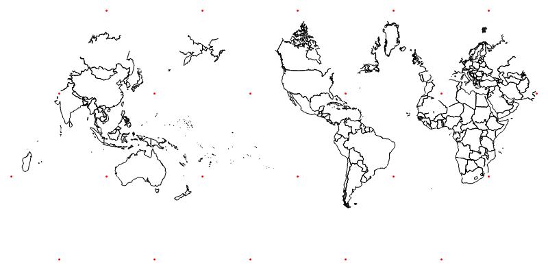
Just cut the shape out, fold between the red dots which are the vertices, and tape it together.
Does anyone know how to find a map of the Moon or Mars or Pluto?


