1. Stippling drawing -- an introduction
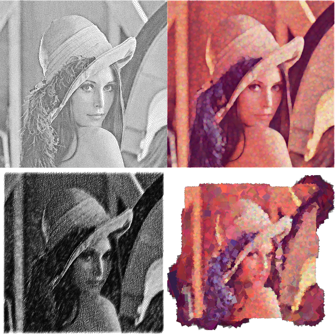
Stippling is a kind of drawing style using only points to mimic lines, edges and grayscales. The entire drawing consists only of black points on a white background. The density of the points gives the impression of grayscale shading.
Back in 1510, stippling was first invented as an engraving technique, then became popular in many fields because of its requirement of just one color of ink. The style influence widely beyond engraving. We can see many technical illustrations done by it, especially in math and mechanics books. Even today many people are interested in it, and archaeologists, geologists and biologists are still using it in field works.
On the art side, stippling shows interesting relation with the divisionism and pointillism, which both belong to the neo-impressionism.
In the domain of so-called non-photorealistic computer graphics, stippling is one of the basic artistic painting style, and can be used as the foundation of many other styles such as mosaic, stained glass, hatching, etc. (Non-Photorealistic Computer Graphics, Thomas Strothotte, Stefan Schlechtweg; The Algorithms and Principles of Non-photorealistic Graphics, Weidong Geng)
2. The essential properties of a "good" stippling
2.1 Well-spaced points
When using points to approximate a grayscale, a random set of points with uniform distributuion is usually not good enough. To illustrate, both images below have 63024 points, but the one on the right is a good stippling (or usually called well-spaced). The one on the left has too many unwanted small artifacts -- clumps and voids do not exist in the original image. (And please be patient, we'll talk about how to generate the "good" one in the next section:)
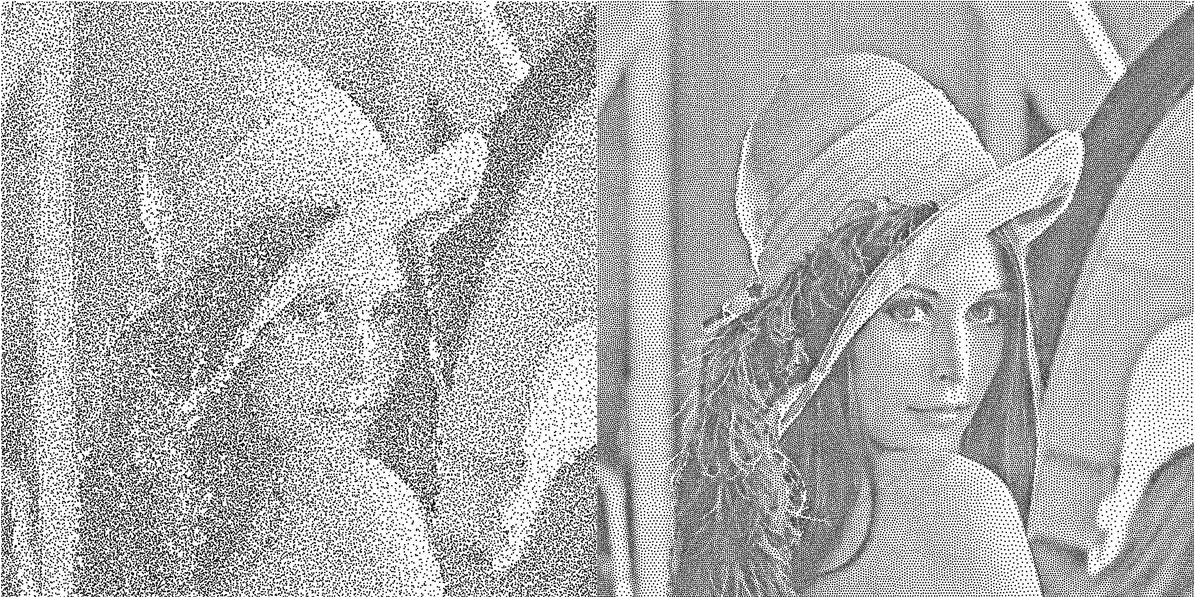
It can be seen that there are too many unwanted small artifacts in the former one -- clumps and voids that do not exist in the original image.
The phenomenon can be seen even more clearly in the uniform grayscale case:
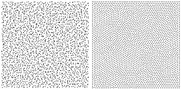
I hope it's plain to see, that in the stippling graphics, the distance between any point and the one nearest to it is nearly a constant. So it looks like we found the essential property of a "good" stippling.
But wait... What about the Lena example? Clearly it's "good" ( if you allow me to say so) but the distances between closest points are various.
It turns out we just need to take one more step to notice that the constant distance implies equilateral triangles:
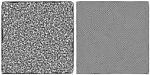
So the so-called good or well-spaced property can be described more precisely as:
The cells of the Delaunay mesh induced by the points are as equilateral triangles as possible.
The statement can be confirmed by the statistics on the set of interior angles of all the cells
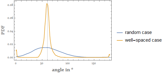
2.2 Another (equivalent) definition
There is still another view point to judge if the positions of the points are good or not.
Consider the same blur taken on all the three Lena images: the original one, the random points one and the well-spaced one:
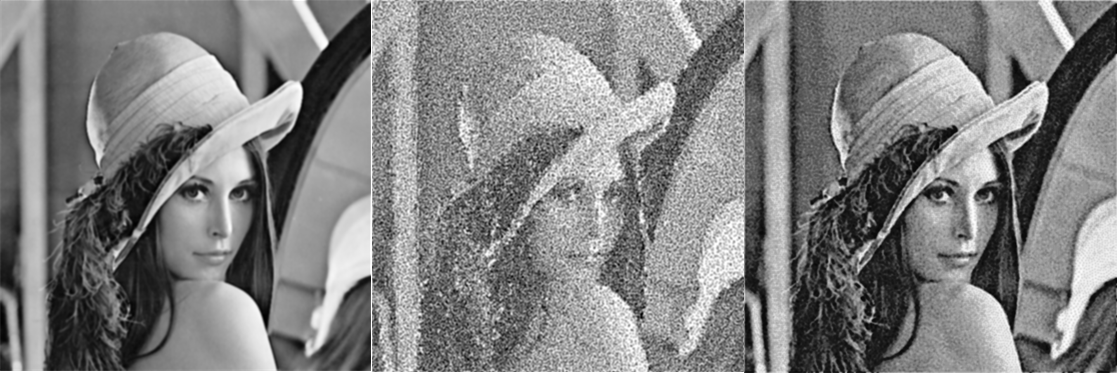
The so-called projection algorithm looks for a point distribution, when convolved with a certain kernel h, which is as the same as the one obtained by convolving the original image with the same h. We are not going to talk about the details here. Readers who are interested in it can refer to the mentioned paper.
3. Stippling of a uniform area -- centroidal Voronoi diagram approach
Now let's do the real fun :)
For an easy start we consider the stippling technique for a uniform area (i.e. an area with constant grayscale). There is a de facto standard method for it called centroidal Voronoi diagram (CVD) which is usually generated by the Lloyd's algorithm.
Basically, the algorithm acts as the following relaxation steps:
Generate $n$ random points inside the interested region
Generate the Voronoi diagram of the $n$ points
Find the centroid (i.e. center of mass) of each Voronoi cell
Use the $n$ centroids as the resulting points
If satisfied, algorithm stop, else goto step 1
Here the key techniques are the Voronoi diagram generation and the centroid finding. The former one is a perfect match for the bounded version of the built-in function VoronoiMesh. The latter one, as the Voronoi cells for a closed region are always closed convex polygons, has a simple formula.
Suppose the cell is defined by $n$ vertices ordered (counter-)clockwise $\{\boldsymbol{P}_1=(x_1,y_1),\boldsymbol{P}_2=(x_2,y_2),\dots,\boldsymbol{P}_n=(x_n,y_n),\boldsymbol{P}_{n+1}=(x_1,y_1)\}$, then its centroid $\boldsymbol{C}$ can be determined as follwing Eq. 1:
$$\left\{\begin{eqnarray} \boldsymbol{C}&=&\frac{1}{6A}\sum_{k=1}^n (\boldsymbol{P}_i+\boldsymbol{P}_{i+1})\,\left|\begin{matrix}x_i&y_i\\x_{i+1}&y_{i+1}\end{matrix}\right|\\ A&=&\frac{1}{2}\sum_{k=1}^n \left|\begin{matrix}x_i&y_i\\x_{i+1}&y_{i+1}\end{matrix}\right| \end{eqnarray}\right.$$
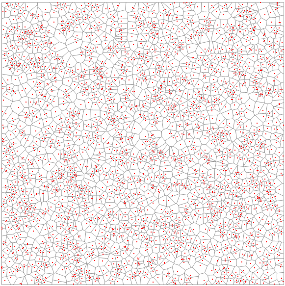
As a test we generate 2500 uniformly distributed random points in a square region $[-1,1]\times[-1,1]$:
initPts = RandomPoint[Rectangle[{-1, -1}, {1, 1}], 2500];
whose Voronoi diagram is:
VoronoiMesh[initPts, {{-1, 1}, {-1, 1}}] //
   Graphics[{
               GrayLevel[.6],
               Line[Identity @@@ MeshPrimitives[#, 1]],
               Red, AbsolutePointSize[2],
               Point[initPts]
            }] &
The Lloyd's algorithm can be expressed as the following findCentroid function:
Clear[findCentroid]
findCentroid[p : Polygon[{{__Real} ..}]] :=
        Module[{pts = p[[1]], pairs, dets, area},
               pairs = Partition[pts, 2, 1, {1, 1}];
               dets = Det /@ pairs;
               area = 1/2 Plus @@ dets;
               dets.(Plus @@@ pairs)/(6 area)
              ]
The cell Polygon-s of the Voronoi mesh can be extracted with MeshPrimitives[...,2], which then should be piped to the findCentroid to complete one iteration:
Module[{vm},
        Function[pts,
                 vm = VoronoiMesh[pts, {{-1, 1}, {-1, 1}}];
                 findCentroid /@ MeshPrimitives[vm, 2]
                ]@initPts
      ];
Now we are ready to animate the first 50 iteration results to give a intuitive feeling about the CVD:
intermRes =
            Module[{vm},
                NestList[
                    Function[pts,
                        vm = VoronoiMesh[pts, {{-1, 1}, {-1, 1}}];
                        findCentroid /@ MeshPrimitives[vm, 2]
                        ],
                    initPts,
                    500
                    ]
                ]; // AbsoluteTiming
refinedPts = intermRes[[-1]];
allframes =
        Function[pts,
                VoronoiMesh[pts, {{-1, 1}, {-1, 1}}] //
                    Graphics[{
                                GrayLevel[.6],
                                Line[Identity @@@ MeshPrimitives[#, 1]],
                                Red, AbsolutePointSize[2],
                                Point[pts]
                                }, ImageSize -> 600] &
                ] /@ intermRes[[;; 50]];
ListAnimate[allframes, 24, DisplayAllSteps -> True, AnimationRepetitions -> 1]
{197.984, Null}
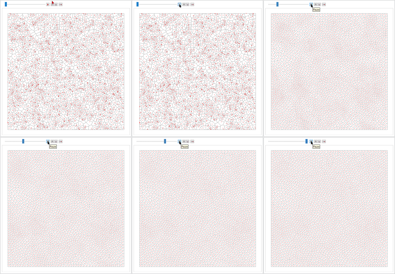
There are various ways to show the difference between the points distributions before and after the process.
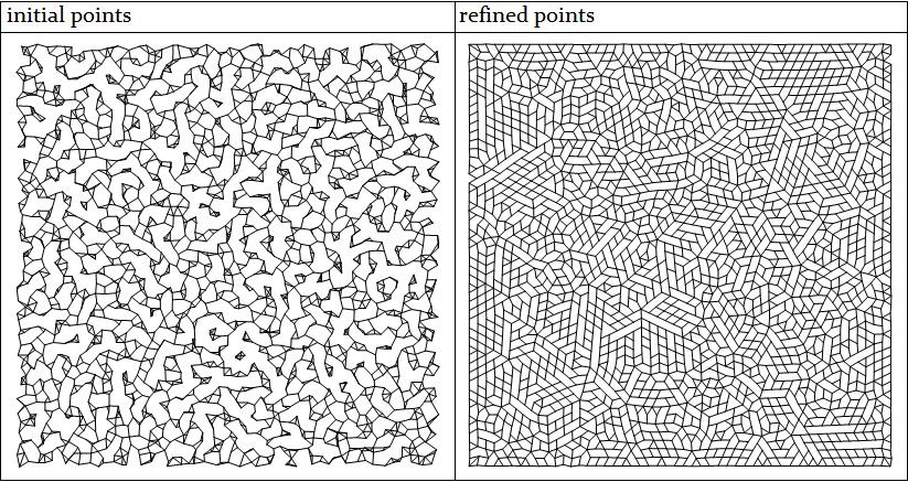
For example we can use NearestNeighborGraph to illustrate the connectivities of them, which will highlight the unwanted voids in the former case:
MapThread[
        Function[{pts, label},
            Graphics[
                    Line[EdgeList[NearestNeighborGraph[pts, 3]] /.
                            UndirectedEdge -> List], ImageSize -> 400] //
                {Style[label, 20, FontFamily -> "Constantia"], #} &
            ],
        {{initPts, refinedPts}, {"initial points", "refined points"}}
        ] // Grid[# // Transpose, Alignment -> Left, Frame -> All] &
Or as having been shown in the previous section, we can compare the statistics of the interior angles:
Plot[
    Evaluate[MapThread[
            Legended[PDF[KernelMixtureDistribution[#1], ?],
                    Style[#2, 15]] &,
            {
                (
                            # // DelaunayMesh // MeshPrimitives[#, 2] & //
                                    Function[pts,
                                                VectorAngle[#2 - #1, #3 - #1]/Degree & @@@
                                                    Partition[pts, 3, 1, {1, 1}]] @@@ # & // Flatten
                            ) & /@ {initPts, refinedPts},
                {"initial points", "refined points"}
                }]],
    {?, 0, 180},
    PlotRange -> All, GridLines -> {{60}, None}, Frame -> True,
    FrameLabel -> (Style[#, Bold, 15] & /@ {"angle in °", "PDF"})
    ]

To give another intuitive impression on the "well-spaced" property from a different point of view, we compare the discrete Fourier transformation of the initial points with the one of the refined points:
MapThread[
        Function[{pts, label},
            Graphics[{AbsolutePointSize[0], Point@pts}] //
                                                            Rasterize[#, ImageSize -> {701, 701}] & // Binarize //
                                                    ColorNegate //

                                                Function[img,
                                                    ImageMultiply[img,
                                                        DiskMatrix[.4 ImageDimensions[img],
                                                                ImageDimensions[img]] // Image]] //
                                            ImageData // # - Mean[Flatten@#] & //
                                    Fourier // Abs // Rescale //
                        RotateRight[#, Floor[Dimensions[#]/2]] & //
                    Image[1.2 - (1 - #)^5, "Real", ImageSize -> 400] & //
                {Style[label, 20, FontFamily -> "Constantia"], #} &
            ],
        {{initPts, refinedPts}, {"initial points", "refined points"}}
        ] // Grid[#//Transpose, Alignment -> Left, Frame -> All] &
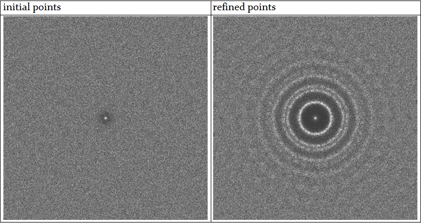
It can be clearly seen that in the refined points' case, we effectively achieved both isotropism and low-stop filter, which is another facet of view to understand the term well-spaced. Note that the property is also related to the concept of "colors" of noise.
4. Stippling of a non-uniform area
So far we only talked about the method for stippling a uniform area. But how about a non-uniform area, like the Lena example?
The Lloyd's algorithm described above can not be directly adapted here without modification, as it always smoothes out the distribution, results a uniform CVD. So how can we generalize it to non-uniform case?
4.1 Approach using the conformal mapping
Recall that we were looking for a Delaunay mesh with cells that resembles equilateral triangles as much as possible, one thing that immediately came to our mind is the conformal map which transforms between two spaces while preserving angles locally. Thus a good stippling on a uniform area is guaranteed to be mapped to a good one on a specified non-uniform area.
A simple example of conformal map is a complex holomorphic function $f$, say $f(z)=(z-z^2/2)\,\exp\left[-(z-1)^2/5\right]$:
cmfunc = Compile[{{z, _Complex}},
                 Module[{w = 1. I},
                        w = (z - 1/2 z^2) Exp[-((z - 1)^2/5)];
                        {Re@w, Im@w}
                       ],
                 RuntimeOptions -> "Speed",
                 RuntimeAttributes -> {Listable},
                 Parallelization -> True
                ];
which transforms the stippling points refinedPts in the uniform square $[-1,1]\times[-1,1]$ to a new points distribution transPts:
transPts = refinedPts.{1, I} // cmfunc;
transPts // Graphics[{AbsolutePointSize[2], Point@#}] &
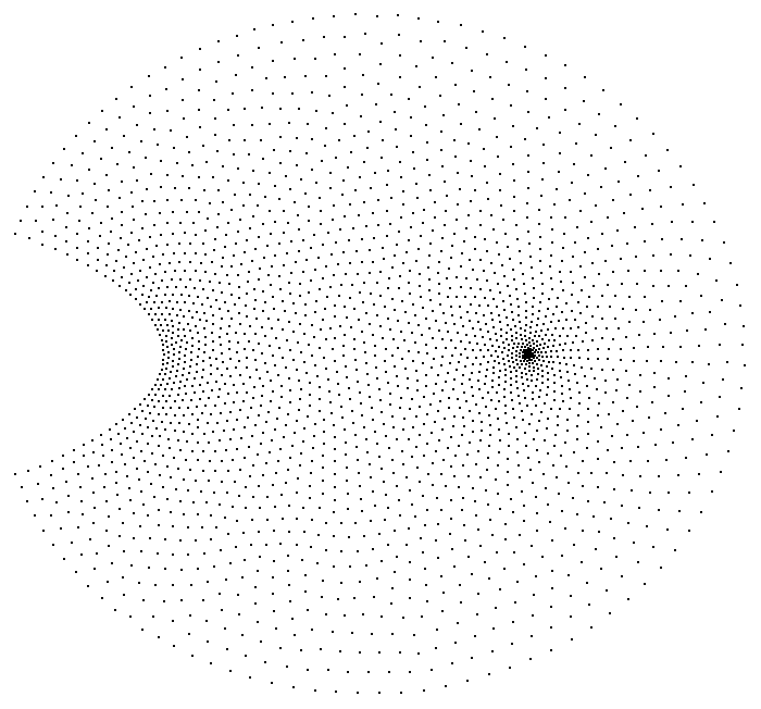
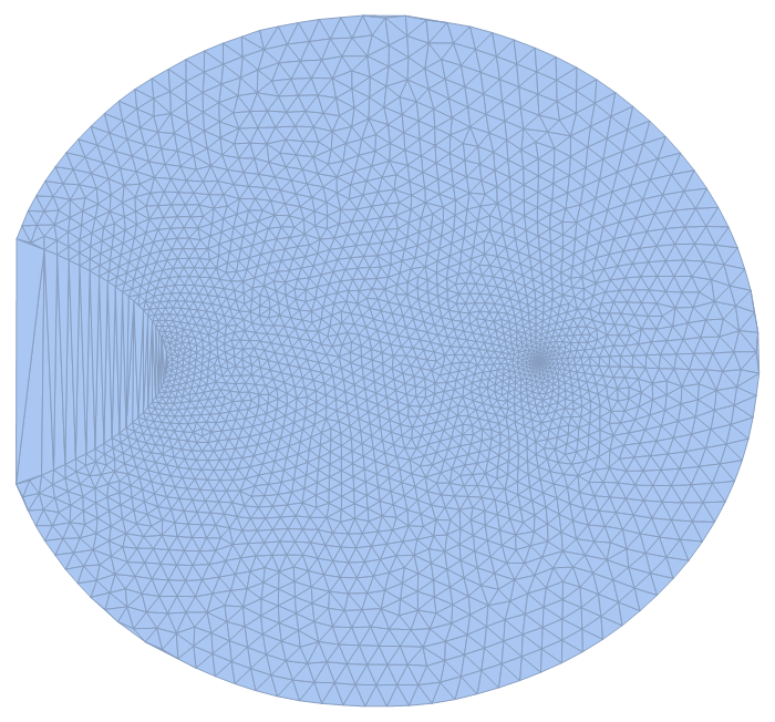
The result looks very nice in the sense of "well-spaced", which can also be confirmed with the Delaunay mesh, Voronoi mesh and its connectivity:
transPts // DelaunayMesh
Module[{vm = VoronoiMesh[refinedPts, {{-1, 1}, {-1, 1}}]},
    Graphics[GraphicsComplex[
            (Identity @@@ MeshPrimitives[vm, 0]).{1, I} // cmfunc,
            vm // MeshCells[#, 1] & // Line[Identity @@@ #] &
            ]]
    ]
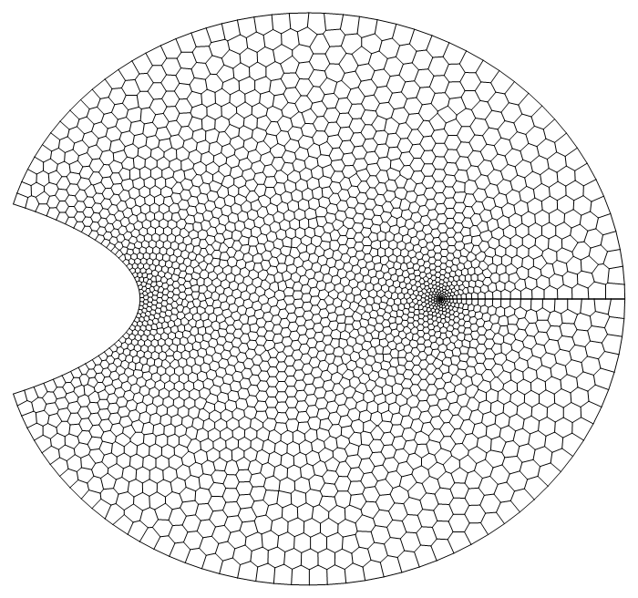
transPts // NearestNeighborGraph[#, 3] & //
                EdgeList // # /. UndirectedEdge -> List & // Line // Graphics
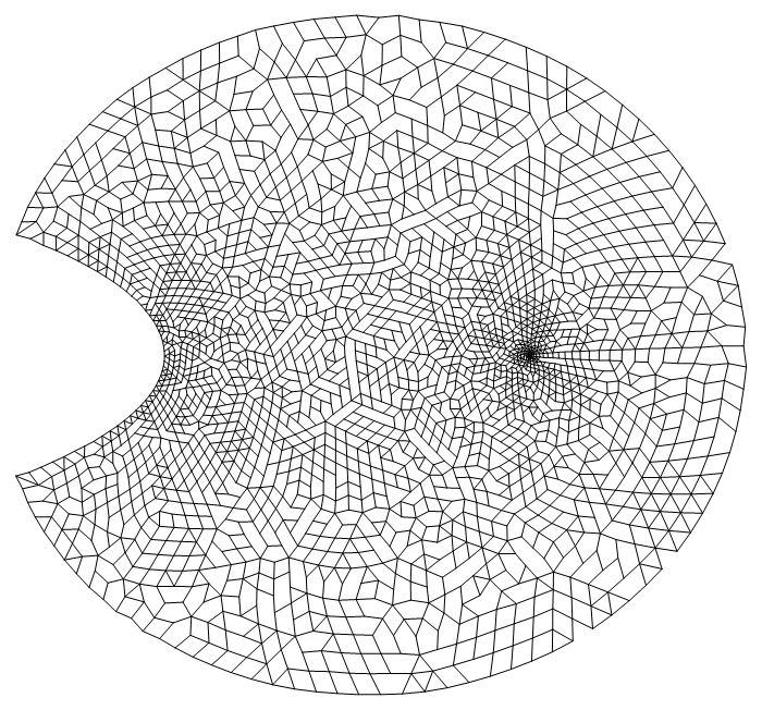
So far so good. However, this theoretically elegant approach is not easily generalizable. To find the right $f$ for an arbitrary target distribution will need sophisticated mathematical skill. Again we are not going to talk about the details here. For readers who are interested in it, there is a whole dedicated research field called computing conformal mapping.
4.2 Approach using the weighted Voronoi diagram
Despite the elegance of the conformal mapping, the popular method for stippling non-uniform area comes from a modification of the CVD, which is called the weighted centroidal Voronoi diagram (A. Secord. Weighted Voronoi stippling. In Proceedings of the second international symposium on Non-photorealistic animation and rendering, pages 37-43. ACM Press, 2002.) (A. Secord. Random Marks on Paper, Non-Photorealistic Rendering with Small Primitives, Thesis for the Degree of Master of Science, 2002).
The algorithm is similar to the Lloyd's algorithm, only in step 3, when looking for the centroid of the Voronoi cell, a variable areal density $\rho(\boldsymbol{P})$ is considered, which is proportional to the grayscale at the location $\boldsymbol{P}$. Thus instead of using Eq. 1, we shall calculate the centroid according to the following definition (Eq. 2):
$$\boldsymbol{C}_{\text{Cell}(\boldsymbol{P})} = \frac{\int_{\boldsymbol{x}\in\text{Cell}(\boldsymbol{P})}\boldsymbol{x}\rho(\boldsymbol{x})\,\mathrm{d}\boldsymbol{x}}{\int_{\boldsymbol{x}\in\text{Cell}(\boldsymbol{P})}\boldsymbol{x}\,\mathrm{d}\boldsymbol{x}}$$
Clearly the integrations are much more time-consuming than Eq. 1. In his paper and master thesis Secord presented an efficient way to compute them, which involves a precomputation of certain integrations. However, I noticed (without theoretical proof) that the weighted CVD can be sufficiently approximated in a much cheaper way if we accept a compromise not to stick to the exact formula (i.e. Eq. 2) of centroid but only to emphasis the core idea of choosing $\boldsymbol{C}$ closer to points with larger weights.
The new idea is simple. For a cell of $n$ vertices $\{\boldsymbol{P}_1,\boldsymbol{P}_2,\dots,\boldsymbol{P}_n\}$, the algorithm acts as follows:
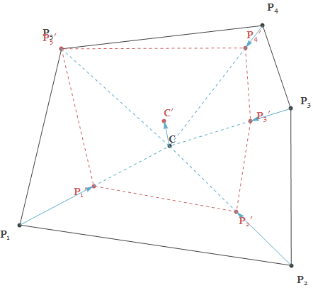
Compute the geometric centroid $\boldsymbol{C}$
Compute the weights of the vertices as $\{w_1,\dots,w_n\}$
Compute normalized weights as $W_k = \frac{w_k}{\max(w_1,\dots,w_n)}$
For every vertex $\boldsymbol{P}_k$, move it along $\overrightarrow{\boldsymbol{C}\boldsymbol{P}_k}$ with factor of $W_k$ to new position $\boldsymbol{P}_k'$ (So vertex with largest weight does not move, vertex with smallest weight moves most)
Compute the geometric centroid $\boldsymbol{C}'$ of the new cell defined by $\{\boldsymbol{P}_1',\dots,\boldsymbol{P}_n'\}$ as the final result
Note that the convergency of our simplified algorithm is not obvious, so it might be wise to do an "early stop" during iteration.
Written in the Wolfram Language, it's this findCentroidW function:
Clear[findCentroidW]
findCentroidW[p : Polygon[{{__Real} ..}], densityFunc_] :=
    Module[{cent, pts = p[[1]], wlst},
           wlst = #/Max[#] &[densityFunc @@@ pts];
           cent = findCentroid[p];
           cent + findCentroid@Polygon@MapThread[#2 (#1 - cent) &, {pts, wlst}]
          ]
Numerical experiments show that this approximation gives fairly good results. In the next section we'll demonstrate its application on the Lena image.
4.3 Numerical experiment on Lena
In this section we test our non-uniform stippling method on the famous Lena's photo.
First let's import the original image. We'll keep both the grayscale and color versions for later use in the artistic rendering section:
imgOrigColored = ExampleData[{"TestImage", "Lena"}];
imgOrig = imgOrigColored // ColorConvert[#, "Grayscale"] & // ImageAdjust;
For Interpolation's convenience, we'll use ColorNegate. For a better visual feeling, we enhance the edges with large gradient:
img = Function[img,
                 ImageAdd[ImageMultiply[img, # // ColorNegate], #] &[
                             GradientFilter[img, 1] // ImageAdjust[#, {2, 2, 1}] &
                            ]
              ][imgOrig // ColorNegate]
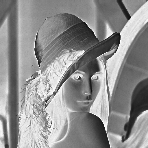
The image coordinate is rescaled to the rectangle region $[-1,1]\times[-1,1]$ for personal convenience and Interpolation-ed to get a smooth description of the grayscale field:
densityFunc =
        img // Reverse[ImageData[#, "Real"]] & // Transpose // Function[array,
                        Module[{dim = Dimensions@array},
                            MapIndexed[{(1 + dim - 2 #2)/(1 - dim), #1} &, array, {-1}]]
                        ] // Flatten[#, 1] & // Interpolation;
To have a good initial points distribution, we would like to sample points so the local density is proportional to the local grayscale (though we don't need to have this precisely, as the weighted Voronoi process will anyway smooth the distribution.) So taking advantage of ContourPlot, we generate a few regions according to the level set of the densityFunc:
levelRegions =
            Module[{ctplot, pts, polys},
                ctplot =
                    ContourPlot[densityFunc[x, y], {x, -1, 1}, {y, -1, 1},
                        Contours -> 10];
                {pts, polys} =
                    Cases[ctplot, GraphicsComplex[pts_, e_, ___] :> {pts,
                                    Cases[e, GraphicsGroup[r : {__Polygon}] :> r, ?]
                                    }, ?][[1]];
                BoundaryDiscretizeGraphics[GraphicsComplex[pts, #]] & /@ polys
                ]; // AbsoluteTiming
{111.862, Null}
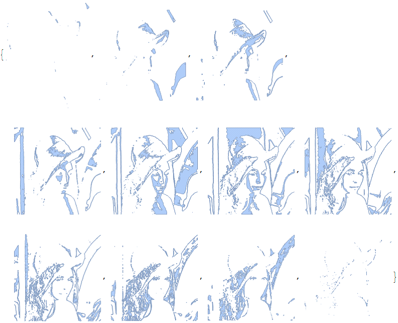
For each region in levelRegions, we sample points inside it on regular grid, with area of the grid cell inversely proportional to the level counter of the region. Notice the regular grid can be a steady state of our algorithm, to ensure a isotropic result, initial randomness is needed. For that purpose we add dithering effect on the points, with its strength specified by a parameter $0\leq\kappa\leq 1$ where $0$ gives no dithering while $1$ gives a globally random distribution:
Clear[ditherFunc]
ditherFunc[pts_, width_, ?_: .5] :=
    pts + ? width/2 RandomReal[{-1, 1}, {Length@pts, 2}]

levelPts =
            Module[{baseGridWidth = 1/50., width, num, min = -1,
                    max = 1, ? = 1},
                MapIndexed[
                    Function[{region, idx},
                        width = baseGridWidth/Sqrt[idx[[1]]];
                        num = Ceiling[(max - min)/width];
                        Tuples[Range@num, 2] //
                                    Rescale[#, {1, num}, {min + width/2, max - width/2}] & // N //

                            ditherFunc[Select[#, RegionMember[region]], width, ?] &
                        ],
                    levelRegions,
                    {1}]
                ]; // AbsoluteTiming
initPts = levelPts // Join @@ # &;
{15.3046, Null}
The total number of points we sampled is huge:
initPts // Length
63024
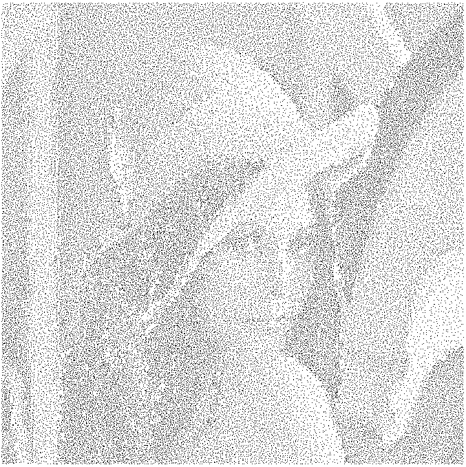
But their quality is poor:
Graphics[{AbsolutePointSize[0], Point@initPts}]
Now we perform the weighted Voronoi relaxation process, which is similar to the one in the uniform case, though the computation is a bit slow due to the amount of points:
refinedPts = Module[{vm},
                Nest[
                    Function[pts,
                        vm = VoronoiMesh[pts, {{-1, 1}, {-1, 1}}];
                        findCentroidW[#, densityFunc] & /@ MeshPrimitives[vm, 2]
                        ],
                    initPts,
                    30
                    ]
                ]; // AbsoluteTiming
{1106.06, Null}
In spite of only 30 iterations, the result is in my opinion fairly good (Note that some visual artifacts in the following image is due to the rasterizing process during display, try right-click and "open image in new tab"):
Graphics[{AbsolutePointSize[0], Point@refinedPts}]

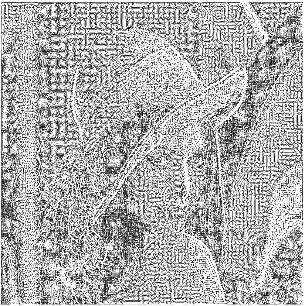
The pattern of the connectivity rather interestingly forms some kind of self-similar multi-resolution tiles:
refinedPts // NearestNeighborGraph[#, 2] & //
                EdgeList // # /. UndirectedEdge -> List & // Line // Graphics
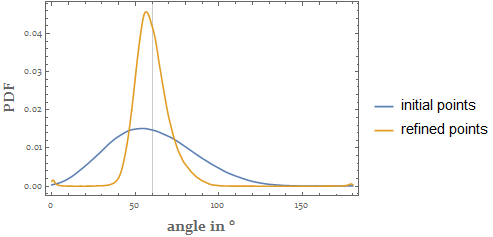
Statistics on the interior angles of the corresponding DelaunayMesh indicates we have indeed achieved the well-spaced distribution:
Plot[
    Evaluate[MapThread[
            Legended[PDF[KernelMixtureDistribution[#1], ?],
                    Style[#2, 15]] &,
            {
                (
                            # // DelaunayMesh // MeshPrimitives[#, 2] & //
                                    Function[pts,
                                                VectorAngle[#2 - #1, #3 - #1]/Degree & @@@
                                                    Partition[pts, 3, 1, {1, 1}]] @@@ # & // Flatten
                            ) & /@ {initPts, refinedPts},
                {"initial points", "refined points"}
                }]],
    {?, 0, 180},
    PlotRange -> All, GridLines -> {{60}, None}, Frame -> True,
    FrameLabel -> (Style[#, Bold, 15] & /@ {"angle in °", "PDF"})
    ]
5. Artistic styles based on stippling
5.1 Hatching
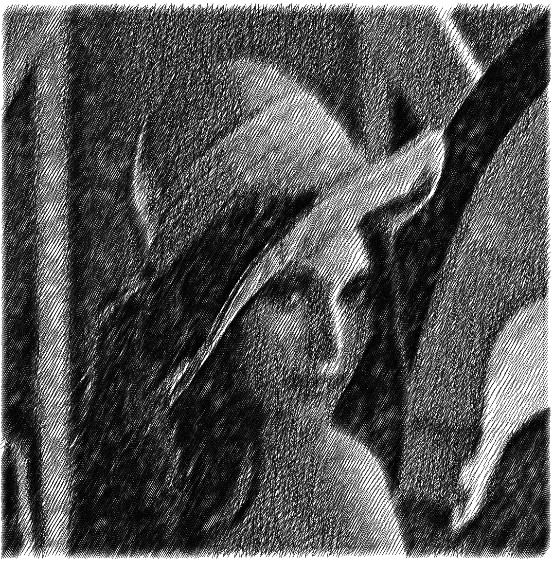
As we mentioned in the introduction, some artistic rendering effects can be simulated based on the stippling result. One of them is hatching, for our example which will act like a pencil sketch. The lengths and orientations of the strokes are controled by densityFunc i.e. local grayscale, while the positions of the them are controled by the stippling points. Note there are artifacts in the dark regions due to our naïve approach:
Module[{strokeLength, strokeOrient, dens, stroke},
    Function[{x, y},
                    dens = densityFunc[x, y];
                    strokeLength = .03 dens^.3 (1 + .1 RandomReal[{-1, 1}]);
                    strokeOrient = ?/
                            3 + ?/6 (1 - (2 dens - 1)^2)^20 RandomReal[{-1, 1}];
                    stroke = strokeLength Through[{Cos, Sin}[strokeOrient]];
                    {{x, y} - stroke, {x, y} + stroke}
                    ] @@@ refinedPts // Line // Graphics[{AbsoluteThickness[0], #}] &
    ]
5.2 Pointillism
Another styling is the simulation of the pointillism.
For this simulation, we need to take care of the colors:
imgColorChannels = imgOrigColored // ColorSeparate[#, "RGB"] &;
densityFuncColorChannels =
        Function[img,
                img // Reverse[ImageData[#, "Real"]] & // Transpose //
                            Function[array,
                                Module[{dim = Dimensions@array},
                                    MapIndexed[{(1 + dim - 2 #2)/(1 - dim), #1} &, array, {-1}]]
                                ] // Flatten[#, 1] & // Interpolation] /@ imgColorChannels;
We add a random deviation of the color on each points:
randomColoredImg =
    {
                                    RGBColor @@ (

                                            Through[
                                                    densityFuncColorChannels[##]] (1 + .3 RandomReal[{-1, 1},
                                                                    3])
                                            ),
                                    Point[{##}]
                                    } & @@@ refinedPts //
                        Graphics[{AbsolutePointSize[0], #} // Flatten,
                                ImageSize -> 1000] & //
                    Rasterize[#, ImageSize -> 1000] & //
                ImageConvolve[#, GaussianMatrix[{10, 1.3}]] & // ImageAdjust //
        ImageCrop
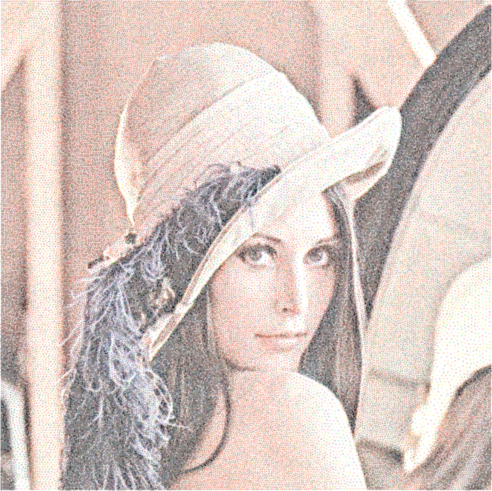
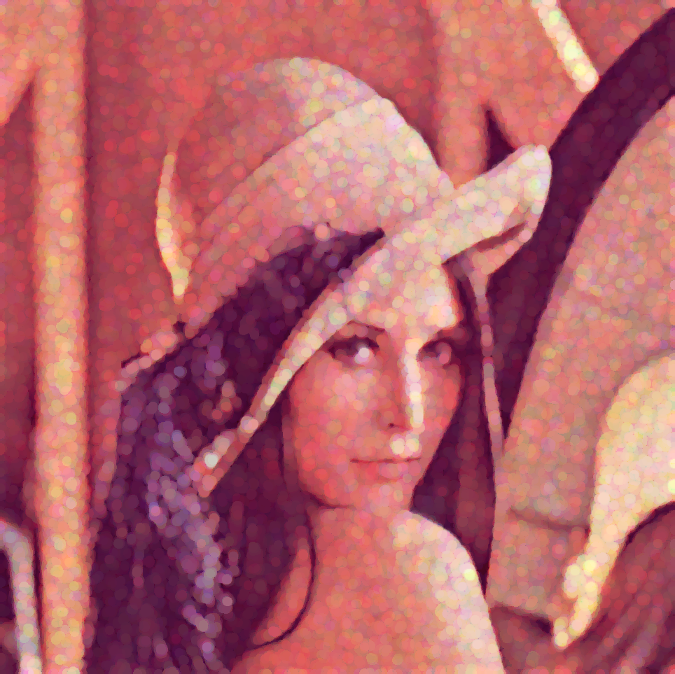
We finalize the process with the morphological Opening operation and match the histogram with the original color image using HistogramTransform:
Opening[randomColoredImg, DiskMatrix[6]] // HistogramTransform[#, imgOrigColored] &
5.3 Pointillism -- another attempt
The rendering in the last section uses strokes with identical size, but in practice it can often vary with some local properties of the targets being drawn. So let's try to include that characteristic here.
For the special property to be reflected, we choose the ImageSaliencyFilter, but it is of course totally fine to choose other ones:
ImageAdjust[
                ImageSaliencyFilter[imgOrigColored, Method -> #]] & /@ {"Itti",
            "IttiColor", "IttiIntensity", "IttiOrientation"};
coarseMask = ImageAdd @@ (Image[#, "Byte"] & /@ %) // Blur[#, 20] &
Like the densityFunc, we interpolation the coarseMask and generate some level regions:
coarseFunc =
        coarseMask // Reverse[ImageData[#, "Real"]] & // Transpose //
                    Function[array,
                        Module[{dim = Dimensions@array},
                            MapIndexed[{(1 + dim - 2 #2)/(1 - dim), #1} &, array, {-1}]]
                        ] // Flatten[#, 1] & // Interpolation;
coarseLevelRegions =
            Module[{ctplot, pts, polys},
                ctplot =
                    ContourPlot[coarseFunc[x, y], {x, -1, 1}, {y, -1, 1},
                        Contours -> 3];
                {pts, polys} =
                    Cases[ctplot, GraphicsComplex[pts_, e_, ___] :> {pts,
                                    Cases[e, GraphicsGroup[r : {__Polygon}] :> r, ?]
                                    }, ?][[1]];
                BoundaryDiscretizeGraphics[GraphicsComplex[pts, #]] & /@ polys
                ]; // AbsoluteTiming
{11.1717, Null}
So now the stippling points can be grouped according to the coarseLevelRegions:
coarseLevelPts = Select[refinedPts, RegionMember[#]] & /@ coarseLevelRegions;
The stroke template is composed with squares centered at the stippling points, with their color determined and randomized in a way similar to that in the last section:
strokeFunc = Function[{pt, size},
            GeometricTransformation[
                    Rectangle[{-1, -1}, {1, 1}],
                    RotationMatrix[
                            RandomReal[?/
                                2]].ScalingMatrix[(1 + .2 RandomReal[{-1, 1}]) size {1, 1}]
                    ] // GeometricTransformation[#, TranslationTransform[pt]] &
            ];
Now we are ready to paint the picture layer by layer. NOTE THAT the following code can be very time-consuming.
coarseLayers =
    Function[{pts, size},
                    {
                                        FaceForm[RGBColor @@ (
                                                    Append[
                                                        (1 + .5 RandomReal[{-1, 1}, 3]) Through[
                                                                densityFuncColorChannels @@ #],
                                                        RandomReal[{.2, 1}]
                                                        ]
                                                    )],
                                        strokeFunc[#, pts]} & /@ pts //
                            Graphics[Flatten@{EdgeForm[], #},
                                    PlotRange -> 1.5 {{-1, 1}, {-1, 1}}] & //
                        Rasterize[#, ImageSize -> 1000, Background -> None] &
                    ] @@ # & /@ ({coarseLevelPts, {.2, .1, .05, .02}}//Transpose)
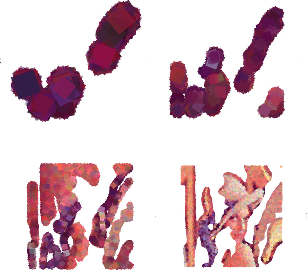
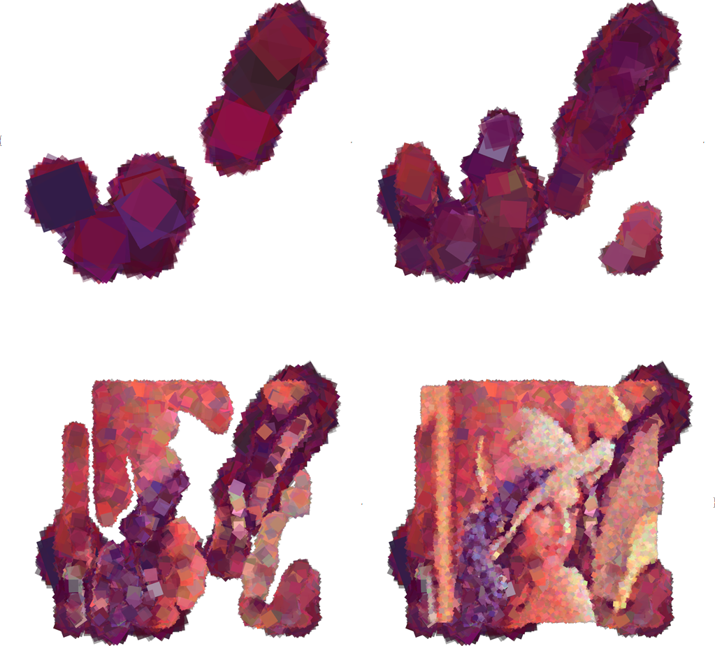
Composing the layers, we get our final "neo-impressionism" result:
composedImg = FoldList[ImageCompose, coarseLayers[[1]], coarseLayers[[2 ;;]]]
composedImg[[-1]] // ImageCrop
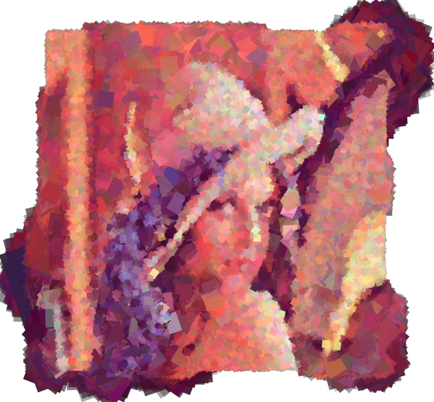
Note the local vivid color blocks especially those at the feather and hat regions, and how the rendering still preserved an accurate scene at the macro-scale. :)
6. Epilogue
In this small writings, we discussed a morden automated method for simulating an ancient art skill called stippling drawing. We also demonstrated how its power can be extended to more advanced artistic renderings. But readers should be reminded that there are other methods for generating the well-spaced point distribution, and there are still many fields related to non-photorealistic computer graphics which are not necessarily related to it. Finally, although not mentioned in this article, the applications of the so-called well-spaced point distribution goes way beyond the examples shown here. The idea can be generalized to high dimensions, and its nice properties makes it an import tool in many scientific feilds, like re-meshing in the finite element method, sparse representation and compressed sensing.