To make a note here, also for myself:
So, when you assume that returns are normally distributed (and you have a clean conscience about that), you mean that
$$\frac{P_1-P_0}{P_0},\frac{P_2-P_1}{P_1},\frac{P_3-P_2}{P_2},...$$
are normally distributed, which is fine! This goes well in line with Geometric Brownian Motion ideas.
But now, when you take the logs of these returns, and sum, what do you actually get?
$$\log \left(\frac{P_1-P_0}{P_0}\right) +\log \left(\frac{P_2-P_1}{P_1}\right) +\log \left(\frac{P_3-P_2}{P_2}\right)+ ... $$
Nothing useful!
What you are looking actually to get is the continuous time return:
$$\log\left( \frac{P_t}{P_0} \right) $$
which can be computed from:
$$\log \left(\frac{P_1}{P_0}\right) +\log \left(\frac{P_2}{P_1}\right) +\log \left(\frac{P_3}{P_2}\right)+ ... $$
But, to get this you need to take logs of (returns + 1).
Now, we can illustrate all this stuff with some Geometric Brownian Motion, which, as I hinted above, assumes that relative changes in asset prices are normally distributed:
$$dS_t=\mu S_tdt+\sigma S_t dW_t $$
Here I have found an example when the seemingly continuous-time return is even lower than -2.
data = RandomFunction[
GeometricBrownianMotionProcess[0, .1, 100], {0, 100, .001}];
ListLinePlot[data, Filling -> Axis, PlotRange -> All,
ImageSize -> Large]
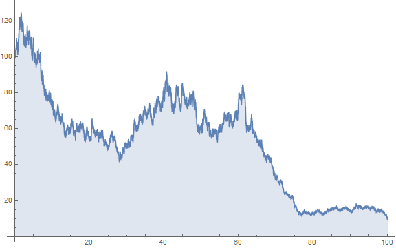
Log[data["Values"][[2 ;;]]/data["Values"][[;; -2]]] // Total

-2.31902
same as:
Log[data["Values"][[-1]]/data["Values"][[1]]]
You need to be very careful how you interpret this result: -2.31902. It is the instantaneous return r multiplied by time t (in our case 100)
So, I can compute the the time t price by the formula:
$$S_t = S_0 e^{r t} $$
And it implies a smooth price journey like this:
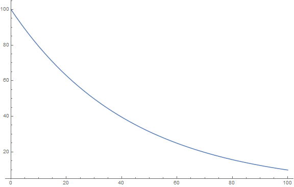
You cannot use it to judge about the holding period return R.
$$R= e^{r t}-1 $$
which under our assumptions will never be below -1. In fact it will never reach -1.


