This is a modified question from the web Q&A community, Zhihu, the Chinese Quora. To run the code in this thread, please download the attachment at the end of the discussion.

Tom and Michael decided to watch Kung Fu Panda 3 on this Saturday. The movie will start at 8:00 pm and they want to meet up at the ticket booth between 7:00 pm to 8:00 pm (arrival time must be in this range). Since neither of them is a time keeper, one is going to buy his own ticket and to head to the theater first if the other is more than 20 min late. Their arrivals are independent.

• Example: Tom arrives first at the ticket booth at 7:30 pm. If Michael arrives at 7:35 pm, he will see Tom at the ticket booth and they buy tickets together. Say, Michael arrives after 7:55 pm, then he will find his own seat inside the theater instead because Tom does not wait for him any more at the ticket booth.

Question:

1. If the likelihood of Tom and Michael arriving at the ticket booth at any time spot is the same (uniform PDF with constant density), what is probablity that they will meet at the ticket booth (ie. they do not have to wait for each other more than 20 min at the ticket booth)?

2. Tom lives in downtown and it is difficult for him to grab a taxi during 7:00 pm - 8:00 pm. The PDF of his arrival time is thus skewed toward 8:00 pm (more likely to arrive at the ticket booth after 7:30 pm than before). Meanwhile Michael's apartment is within 5 min walk distance from the theater in a suburb and he is more likely to arrive the ticket booth before 7:30 pm than after. What is probability that they will meet at the ticket booth (ie. they do not have to wait for each other more than 20 min at the ticket booth)?

Find a solution

This is a very common situation in real life (except in Q2 Michael will be the late dude in general ;-) ) which involves some interesting discussions in the probability theory. Q1 is with a fairly ideal assumption and we will find a rigid solution. Q2 is more or less an open question, leaves us the chance to explore several sets of parameters.

We know both Tom and Michael are bad at punctuality, we can conclude that the probability of Tom waiting for Michael and vice versa are the same. Also to make the problem easy we can set use 1 for the time span (7 pm =0, 8pm =1) and 1/3 for the maximum waiting time (20 min / 60 min = 1/3).

Q1

• Try the Mathematica super function. Just input the following function into the "Probability". 100% black box. Bang! Solution!

Changing max waiting time with step = $1/60\ \text{hr}$ = $1$ min, we can find a profile of the chance of meeting against this change easily. Use the numeric probability finder to speed up the calculation

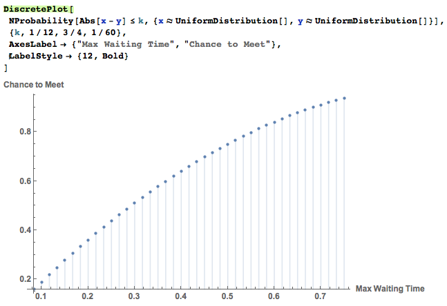
we know the plot makes sense because the longer the two can wait for each other, or tolerate each other, the more chance they can meet at the ticket booth.

• Detailed Analysis

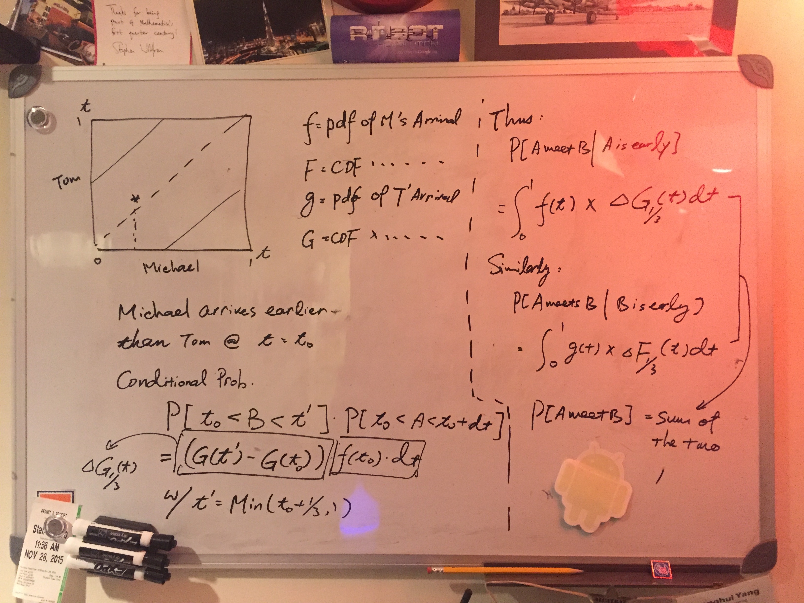
Let's assume Michael arrives first at time $t_{0}$. Therefore Tom must arrive at the ticket booth between $t_0$ and $ \text{Min}[ t_0+1/3 , 1]$ to meet with Michael. This conditional density is thus

$Prob[t_0<T<Min[t_0+1/3,1]]\ \text{Given Michcael arrives at the ticket booth at } t_0$

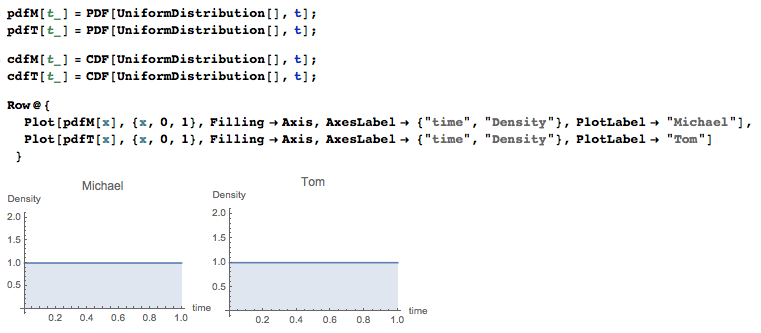
Let pdfM[t] be the PDF of Micheal's arriving time and pdfT[t] be Tom's. By Q1's assumption about the uniformity, we have

The CDF plot of the arrival time for both

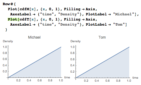
Because the time variable is continuous, the probability of Michael arriving at exactly at $t_0$ is zero. But the probability of arrival between $t_0$ and $t_0 + dt$ is calculable for small dx:

$Prob[t_0<T<t_0+dx] \approx \text{pdfM}[t_0]*dt$

Therefore the probability of their meeting is

$ \text{pdfM}[t_0]*dt*(\text{cdfT}[\text{Min}[t_0+1/3,1]]-\text{cdfT}[t_0]) $

given the independence assumption in the problem. Thus, in the case of Michael being ahead of time, the probability of their meeting is the sum of the probability at all possible value of $t_0$, which is the following integral:

p1=Integrate[pdfM[t]*(cdfT[Min[t+1/3,1]]-cdfT[t]),{t,0,1}] (* result is 5/18 *)

or use the super "Probability" function again

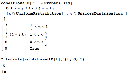
Because of the symmetry and the fact that the two events, Michael awaiting Tom and vice versa, are mutually exclusive, the result is simply

 2*p1 (* result is 5/9 *)

• Graphical Solution

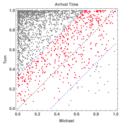
We also have a graphic interpretation of the result above. In the graph below, the X axis denotes the arrival time of Michael and Y axis is that of Tom. There are several characteristic points and lines on the graph.

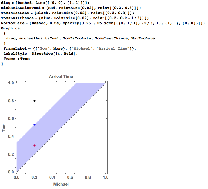
The diagonal line: Michael and Tom arrive at the ticket booth at the same time aka zero waiting time. The line perfectly divides the graph into two regions.

The part above the diagnal is Michael's earliness.The coordinate of red dot is {0.2, 0.3}, which means Michael arrives at about 7:12 pm and Tom is late about 6 min, or arrives at 7:18 pm. This is an acceptable case.The black dot at {0.2,0.8} is an unacceptable case. Tom arrives at 7:48 pm, almost 36 min (> 20 min) late.

The area of the trapzoid can be computed directly or by the subtraction of the upper triangle area from the area of the half square, which is

trapzoidArea = 1/2 - 1/2*(2/3)^2

By symmetry, the probality that we are looking for is

2*trapzoidArea (* result is 5/9*)

• Monte-Carlo Solution

This is quite straight-forward. I generate a bunch of dots {Michaels arrival time, Tom's arrival time} and color-code them according to whether the difference between the two components is greater than $1/3$ or not:

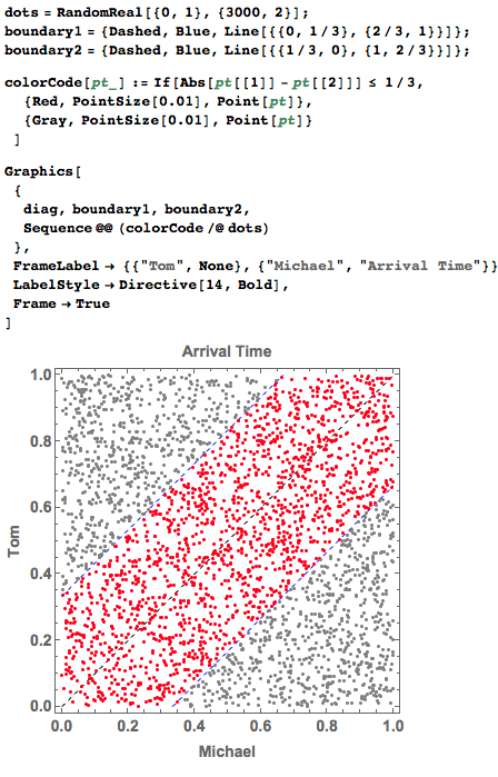
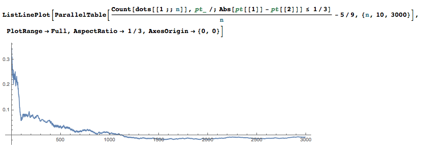
The convergence speed is not good at all since it requires more than 1000 data points to reach a small error region. The algorithm below is just counting the red dots in the graph and compute the portion/ the probability of the two people meeting at the ticket booth.

• Q2

In Q2 we are dealing with the non-uniform distribution. First thing to note is that the symmetry no longer holds. To compute this case we need a generic form of such. In fact, the following code denotes a more general form to the solution of this problem:

NIntegrate[pdfM[t]*(cdfT[Min[t + 1/3, 1]] - cdfT[t]) + pdfT[t]*(cdfM[Min[t + 1/3, 1]] - cdfM[t]),{t, 0, 1}],

Derivation:

I have the following complicated function to handle the plot and computation at the same time.

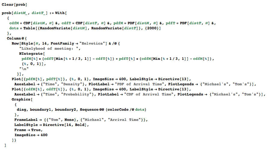
In Q2 we do not have a very specific distribution but we can play around with some build-in Mathematica distribution to find a suitable one. One set of the candidates is

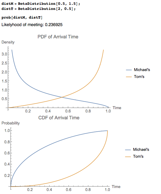
What is the effect of this skewed distribution on our result? the graphics method we used above no longer valid because the dots are skewed. In this case we realize that the area we have computed before is in fact a VOLUME! In the uniform distribution case, the hight/probability density is the same across the domain (and it is exactly 1 because $1 \times 1 \times 1 =1 $, the volume of unit cuboid)

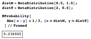
If you are still in a rush to get the answer without wanting to look at the step above, the super function Probability also works. Bang! Solution!

To explore more about how their arrival time density function affects the probability that we are looking for, I played around the with BetaDistribution with more settings:

Block[{distM, distT}, Grid[{
    Table[
     distM = BetaDistribution[k, 1.5];
     distT = BetaDistribution[1.5, k];
     prob[distM, distT],
     {k, {1/2, 1, 2, 4}}]}] // Magnify[#, 0.65] &]

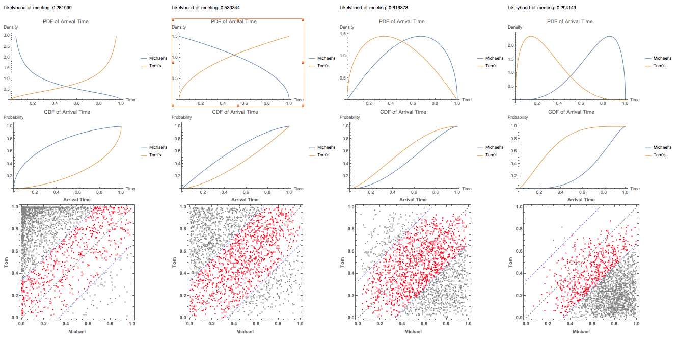
Graphically we can see that if the common area under the PDF's are larger, the more dots sit in the valid zone $ x-1/3 < y < x+ 1/3$. Meanwhile, the more common area under the PDF curve, the smaller the hysteresis shape in the CDF graph (a very general conclusion). One can tell that the more skewed the curve towards the different end of the domain, the less likely the people can meet at the ticket booth.

• The Extra

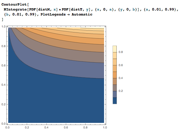
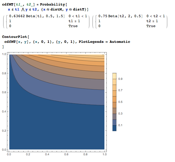
By the assumption the arrivals of the two people are independent, we know that the joint PDF is the product of the two individual PDF's. This is also true for the joint CDF. Graphically we can verify the assertion. Notice that the second takes significantly time to compute:

Attachments: