Hi Craig,

I changed your difference relation slightly so y[n] is a function of in[[n]], otherwise the count on in and out does not match. The technique below uses the difference relation build a sum-of-squares error function between symbolic terms and the list of out values, and then uses FindMinimum to determine parameter values which minimize the error. It's a useful technique.

Best regards, David

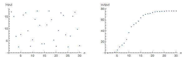
In[1]:= in = {16.969, 15.151, 6.83824, 2.51202, 7.62716, 15.7341, 
   16.6111, 9.15233, 2.76235, 5.4981, 13.9102, 17.392, 11.5535, 
   3.75623, 3.83153, 11.6845, 17.4135, 13.7951, 5.39155, 2.79867, 
   9.28573, 16.6734, 15.6468, 7.50031, 2.50563, 6.96037, 15.2477, 
   16.9184, 9.86588, 2.98251};

In[2]:= out = {0.1, 0.235755, 0.520125, 1.58736, 5.30637, 10.8286, 
   14.5398, 17.9214, 24.4315, 36.8878, 47.4856, 51.8436, 54.3319, 
   57.7956, 63.7485, 68.5763, 70.3306, 71.0822, 71.8903, 73.2932, 
   74.6665, 75.2082, 75.4013, 75.5603, 75.8267, 76.1532, 76.3087, 
   76.3591, 76.3908, 76.4382};

In[3]:= Length /@ {in, out}

Out[3]= {30, 30}

In[4]:= (* mofified to give out[[n]] as a function of in[[n]]*)
y[n_] := y[n] = y[n - 1] (1 + a Exp[-(b in[[n]] + c (n))]);

In[5]:= y[0] = y0; (* to be determined *)

In[6]:= (* sum of squares error from measured out *)
(* to big to print conveniently *)
error = Sum[(y[n] - out[[n]])^2, {n, Length[out]}];

In[7]:= (* the first term of the sum *)
error[[1]]

Out[7]= (-0.1 + (1 + a E^(-16.969 b - c)) y0)^2

In[8]:= (* the second term *)
error[[2]]

Out[8]= (-0.235755 + (1 + a E^(-15.151 b - 2 c)) (1 + 
     a E^(-16.969 b - c)) y0)^2

In[9]:= (* minimize the error *)
sol = FindMinimum[error, {a, b, c, y0}]

Out[9]= {54.7861, {a -> 7.49923, b -> 0.0349481, c -> 0.296997, 
  y0 -> 0.0143244}}

In[10]:= (* a table of calculated out values *)
check = Table[y[n] /. sol[[2]], {n, Length[out]}];

In[11]:= plot = 
 ListPlot[{out, check}, PlotLegends -> {"given", "modeled"}]

Attachments:

David, thank you very much for walking me through the FindMinimum approach to fitting parameters in my model. I played with your nb, and found that it does everything I wanted in terms of setting initial parameter estimates, gradient method, norm function ("error" in your nb). I'm looking at changing my modeling approach based on Sean's considered advice regarding well-known time series models. For now, though, you've provided the solution I was looking for. I appreciate your taking the time to help.

I suggest you have a look at your iter function. y is used as afunction, but nowhere defined. in[[n-1]] is used, which means the lowest value of n that can be used is 2, which will extract the first value of in. out is defined as a function, but out was previously defined as the output list.